Download
1 / 30
300 likes | 337 Views
This study focuses on the use of real-time 3DVAR storm-scale assimilation to improve tornado forecasting accuracy. By assimilating data from multiple sensors, including radar, the study aims to generate probabilistic tornado guidance and track potentially tornadic supercells. The system uses a high-resolution 3D analysis and ensemble forecasts to provide probabilities of hazardous weather. The results show improved forecast skill, with storm tracks and trends predicted up to an hour in advance.

E N D
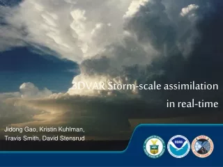
3DVAR Storm-scale assimilation in real-time Jidong Gao, Kristin Kuhlman, Travis Smith, David Stensrud
Convective-scale Warn-on-Forecast Vision Radar and Initial Forecast at 2100 CST Radar at 2130 CST: Accurate Forecast Probabilistic tornado guidance: Forecast looks on track, storm circulation (hook echo) is tracking along centerline of highest tornadic probabilities An ensemble of storm-scale NWP models predict the path of a potentially tornadic supercell during the next 1 hour. The ensemble is used to create probabilistic tornado guidance. Most Likely Tornado Path Most Likely Tornado Path Developing thunderstorm 30% 30% 50% 50% 70% 70% T=2200 CST T=2200 CST T=2150 T=2150 T=2140 T=2140 T=2130 T=2130 T=2120 CST T=2120 CST Stensrud et al. 2009 (October BAMS)
Probabilistic convective-scale analysis and forecast system • High-resolution 3-d analysis produced every 5 min • 1-h ensemble forecasts produced every 5 min • Provides probabilities of hazardous weather • Assimilation of all available observations
Multiple sensors + Denser Observations! Radar #1 Radar #2 Radar #3 4
Near-surface reflectivity Reflectivity @ -20 C Total Lightning Density Max Expected Size of Hail (~6.5 km AGL) Example: Multi-sensor data fields • Show physical relationships between data fields from multiple sensors • Storm tracks and trends can be generated at any spatial scale, for any data fields • Future state predicted through extrapolation shows skill out to about an hour 5
A better alternative? Radar #1 Radar #1 Radar #2 Radar #2 Radar #3 Radar #3 Courtesy Lou Wicker
Single analysis 3D Wind (U/V/W) Solve vorticity equation Not limited by edge of echo Pres/Temp/RH that can also be used to initialize forecast models for Warn-on-Forecast
Radar Data Assimilation Tornado Tracks Dowell and Wicker (2009)
Real-time assimilation / Hazardous Weather Testbed (Spring 2012)
Getting started: R & D goals for Spring 2012 • To create realtime weather-adaptive 3DVAR analyses at high horizontal resolution and high time frequency with all operationally available radar data from the WSR-88D network. • To use the analysis product to help detect supercells and determine if these analyses can improve forecasters awareness of the hazardous weather event.
3D-Var: An Introduction • Given a set of observations and a model of some physical parameters, what does knowledge of observations tell us about the model state? • 3D-Var finds the optimal analysis that minimizes the distance to the observations weighted by the inverse of the error variance J(x) = cost function (to be minimized such that x = xa: ) Xa= optimal analysis of field of model variables Xb= background field Y0= observations H matrix transforms vectors in model space to observation space B = background error covariance R = observational error covariance
3D-Var: An Introduction • The minimum is found by numerical minimization, which is typically an iterative process • Schematic of the cost function minimization in two dimensions. • The minimum is found by performing several searches to move the control variable to areas where the cost-function is smaller, usually by looking at the local slope (the gradient) of the cost-function. Fig. from ECMWF (Bouttier & Courtier)
3D-Var: Advantages • The essence of the 3D-Var algorithm is to rewrite a least-squares problem as the minimization of a cost-function. The method was introduced in order to remove the local data selection in the Optimal Interpolation algorithm, thereby performing a global analysis of the 3-D meteorological fields, hence the name. • For 3D-Var: Observations and model variables can be non-linearly related • There is no data selection – all available data used simultaneously (no jumpiness in boundaries between regions) • 4D-Var is generalized as 3D-var for observations that are distributed in time. • 4D-Var is more complex: needs linearized perturbation forecast model and its adjoint to solve the cost function minimization problem efficiently
Real-time system • 1pm to 9pm daily • 4 floating domains (user-controlled) • 1 km res • 31 vertical levels • 200x200 grid points • 5-min updates • Near-real-time (<5 min latency)
Real-time system • NAM forecast is used for the background field • interpolated to the 3DVAR analysis time • Uses Reflectivity and Radial Velocity from all nearby WSR-88D radars • Cloud analysis • 3DVAR Wind analysis
3D Wind field Max updraft Simulated Reflectivity & 3D Wind Vector
Vorticity Tracks 3DVAR assimilation vorticity track 0-3 km MSL KTLX azimuthal shear track 0-3 km MSL
May 10, 2010 Courtesy NWS-Norman
April 14, 2011 – floating domains working together Floating Domain Vorticity Track (6-hour) Updraft Track (6-hour)
May 16 Hail Storm / OKC Assimilation simulated reflectivity KTLX Reflectivity
Notes • 20 prior cases (from 2010, all of which are supercells) showed: • max W range: 15 to 25 m/s • max Vorticity range: 0.012 to 0.032 s-1 • values seem to vary based on range from radar • More study is needed, here • Trends of vorticity match azimuthal shear • Updraft intensity frequently trends w/ MESH
A typical session • You will use the 3DVAR analysis to help with warning decision assistance. • AWIPS / WarnGen; WDSS-II for some displays • Feedback: • real-time observation / discussion (recorded to EWP blog) • web-based surveys • daily post-mortem discussion
Things to ponder this week • Look long-term (5-10-15 years into the future). • Think about how the 3DVAR storm structure and morphology compare to how you would analyze the data during typical forecast/warning operations in your office. • Consider how storm-scale ensemble prediction will affect warning decision-making and communication of warning information in 10-15 years.
In Conclusion • You are getting the first look at these real-time data! • It’s the start of a > 10-year journey. • Web archive / real-time images: • http://www.nssl.noaa.gov/users/jgao/public_html/analysis/RealtimeAnalysis.htm • http://tiny.cc/3DVAR