Download
1 / 40
400 likes | 531 Views
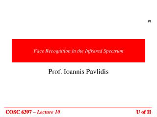
Face Recognition in the Infrared Spectrum. Prof. Ioannis Pavlidis. COSC 6397. U of H. Primary Applications. Biometric Identification Passwords/PINs. Tokens (like ID cards). You can be your own password. Surveillance

E N D
Face Recognition in the Infrared Spectrum Prof. Ioannis Pavlidis COSC 6397 U of H
Primary Applications • Biometric Identification • Passwords/PINs. • Tokens (like ID cards). • You can be your own password. • Surveillance • Off-the-shelf facial recognition system that identifies humans as they pass through a camera’s field of view.
Novel Applications • Wearable Recognition Systems • Adapt to a specific user and be more intimately and actively involved in the user's activities. • Face recognition software can help you remember the name of the person you are looking at. • Useful for Alzheimer's patients. • Smart Systems • Key goal is to give machines perceptual abilities that allow them to function naturally with people. • Critical for a variety of human-machine interfaces.
Why Infrared? Visible cameras sense reflected light Thermal cameras sense emitted radiation • Visible light has no effect on images taken in the thermal infrared spectrum. • Even images taken in total darkness are clear in the thermal infrared.
Why Infrared? (Contd..) • Illumination Invariance • Major problem in visible domain. • Uniqueness and Repeatability • Sense thermal patterns of blood vessels under the skin, which transport warm blood throughout the body. • Remain relatively unaffected by aging. • Even identical twins have different thermograms. • Immune from Forgery • Disguises can be easily detected.
Previous Work • Lot of research was done in the visible band but little attention was given in the infrared spectrum. • Recent reduction in the cost of infrared cameras and availability of large data sets encouraged active research in infrared face recognition. • Low-Level Models • Directly analyze the image pixels and impose probabilities on the features. • Examples are PCA, ICA, and FDA. • Not good in challenging conditions. • High-Level Models • Synthesize images from 3D templates of known objects and impose probabilities on transformations. • Template matching approaches. • Computationally expensive. • Our Proposal • Intermediate model which takes advantage of both Low-Level and High-Level models.
Principal Component Analysis • A D = H x W pixel image of a face, represented as a vector occupies a single point in D2-dimensional image space. • Images of faces being similar in overall configuration, will not be randomly distributed in this huge image space. • Therefore, they can be described by a low dimensional subspace. • Main idea of PCA (cutler96): • To find vectors that best account for variation of face images in entire image space. • These vectors are called eigen vectors. • Construct a face space and project the images into this face space (eigenfaces).
Eigenfaces Approach - Training • Training set of images represented by 1,2,3,…,M • The average training set is defined by Ψ = (1/M) ∑Mi=1i • Each face differs from the average by vector Φi = Γi – Ψ • A covariance matrix is constructed as: C = AAT, where A=[Φ1,…,ΦM] • Finding eigenvectors of N2x N2 matrix is intractable. Hence, find only M meaningful eigenvectors. M is typically the size of the database.
Eigenfaces Approach - Training • Consider eigenvectors vi of ATA such that ATAvi = μivi • Pre-multiplying by A, AAT(Avi) = μi(Avi) • The eigenfaces are ui = Avi • A face image can be projected into this face space by Ωk = UT(Γk – Ψ); k=1,…,M
Eigenfaces Approach - Testing • The test image, Γ, is projected into the face space to obtain a vector, Ω: Ω = UT(Γ – Ψ) • The distance of Ω to each face class is defined by Єk2 = ||Ω-Ωk||2; k = 1,…,M • A distance threshold,Өc, is half the largest distance between any two face classes: Өc = ½ maxj,k {||Ωj-Ωk||}; j,k = 1,…,M
Eigenfaces Approach - Testing • Find the distance, Є , between the original image, Γ, and its reconstructed image from the eigenface space, Γf, Є2 = || Γ – Γf ||2 , where Γf = U * Ω + Ψ • Recognition process: • IF Є≥Өcthen input image is not a face image; • IF Є<ӨcAND Єk≥Өc for all k then input image contains an unknown face; • IF Є<Өc AND Єk*=mink{ Єk} < Өcthen input image contains the face of individual k*
Limitations of Eigenfaces Approach • Variations in lighting conditions • Different lighting conditions for enrolment and query. • Bright light causing image saturation. • Differences in pose – Head orientation • 2D feature distances appear to distort. • Expression • Change in feature location and shape.
IR Face Recognition – Training Phase Compute Offline
Segmentation • Noise in the background may effect the performance of a face recognition system. • Remove the background. • Use thermal information on face to compute the features. • Adaptive Fuzzy Segmentation (kakadiaris02) • Fuzzy affinity is assigned to spels w.r.t. target object spel. • Affinity is computed as weighted sum of the temperature and the temperature gradient in the neighborhood of the target spel. • Minimal user interaction because of dynamically assigned weights.
Segmentation (Contd..) • Fuzzy affinity is calculated by: Weights Spatial Adjacency Temperature Homogeneity Temperature Gradient • Spatial Adjacency:
Segmentation (Contd..) • Temperature homogeneity & gradient: - Temperature of seed c - Temperature of seed d - Mean Temperature - Standard deviation of temperature • Weights: Computed Adaptively
Problem with Single Seed • Temperatures on face are different at different regions. • If a single seed is chosen in a particular region, then the connectivity stretches only along this region and the segmentation goes wrong.
Multiple Seeds Seeds represented by white cross-marks • Solution to this problem is to choose multiple seeds in different regions on face and merge the resulting segmented parts . • Choose a seed pixel on face wherever there is sharp change in gradient. • Works well even when the subject is wearing glasses. • Robust to variation of poses.
Choosing Multiple Seeds 3 4 Move up and pick a seed in pink region (typically forehead) Move up and pick a seed in cyan region (typically forehead) 1 2 Start from center Pixel Move right and pick a seed in blue region (typically right cheek) Move left and pick a seed in blue region (typically left cheek) Move down and pick a seed in pink region Move down and pick a seed in cyan region 6 5
Assumptions • Merge all resultant segmented regions to form final image. ASSUMPTIONS • The center of the image contains the pixel from facial region. • The temperatures at all pixels are mapped between 0 and 255. • If this mapped temperature at a pixel is between 175 - 200, it is classified to be in blue region. • If this mapped temperature at a pixel is between 200 - 225, it is classified to be in pink region. • If this mapped temperature at a pixel is between 225 - 255, it is classified to be in cyan region.
Feature Extraction • The segmented facial image is divided into its spectral components using Gabor filters. • The resultant Gabor filtered images are modeled using Bessel models. • The Gabor filter bank is given by: Scale Orientation
Gabor Filter Bank Different Scales • Example Gabor filter bank with 3 scale values and 4 orientation values: Different Orientations
Spectral Components Scale = 1, 2, 3 Orientation 150 Original Image Spectral Components
Bessel Parameters • Each segmented image in training set is convolved with the filters in Gabor filter bank to obtain Gabor filtered images. • The filtered images are modeled using Bessel parameters: SK – Sample Kurtosis SV – Sample Variance Shape Parameter Scale Parameter
Sample Variance and Kurtosis • Sample Variance is the measure of the “spread” of the distribution. • Sample Kurtosis is the measure of the “peakedness” or “flatness”. Sample Kurtosis,
Bessel Model • Using the bessel parameters p and c, the filtered image I(j)(x,y) is modeled as: Modified Bessel Function of Second Kind Normalizing constant (p) is gamma function Iv(z) is modified bessel function of first kind given by:
Bessel Model Estimated histogram using Bessel model Observed histogram of Gabor filtered Images
Performance of Bessel K Forms • Kullback-Leiber divergence: KL div=0.0013 KL div=0.0027 KL div=0.0055 KL div=0.0058 – observed marginal density – Estimated Bessel Form
Comparing IR Images • Images modeled into Bessel parameters can be compared by: • L2-metric between two Bessel forms f(x;p1,c1) and f(x;p2,c2) in D:
Hypothesis Pruning • Applying a high-level classifier on entire database is computationally very expensive. • Pruning of hypotheses can be achieved by using Bessel parameters (anuj01). • Helps in short listing best matches. • Bessel parameters for images in database can be computed offline which helps in saving a lot of computation time.
Hypothesis Pruning (Contd..) • Define a probability mass function on the database A: (D=0.3 for Equinox dataset) (p(j)obs,c(j)obs) – observed Bessel parameters for test image I(j) (p(j),s,c(j),s) – estimated Bessel parameters which can be computed offline • Images in database A with P1(|I) greater than a specific threshold value are short listed as best matches.
Hypothesis Pruning (Contd..) Pruned Hypothesis • Shortlist the subjects of A with P1(/I) greater than a specific threshold: Elements of A Exact Match
Pruning Algorithm Images with this value greater than a threshold are shortlisted
Test Image Training Image at Pose 's' Classification Aprori Likelihood • Bayesian target recognition (anuj00) searches for the target hypothesis with largest posterior probability given by: • Likelihood: : Variance of test image d : dimension of image (2 in this case) • Apriori is same for all images in database (for database of n images, it is 1/n for each image).
Experiments Sample Images • Equinox Database: www.equinoxsensors.com • Image frame sequences were acquired at 10 frames/sec while the subject was reciting the vowels ‘a’,’e’,’i’,’o’,’u’. Experimental Setup
Results – ROC Curves Correct Positive : Test image is in the database and is correctly recognized. False Positive : Test image is not in the database, but is recognized to be an image of the database Negatives : Test images that are not in the database.
Conclusion • We came up with a face recognition approach which is computationally inexpensive and at the same time good in challenging conditions. • The features of all images in database can be computed offline and stored for future use. This saves lot of computation time. • We improved the performance of classifier by removing background noise of pruned hypothesis using adaptive fuzzy connectedness based image segmentation.
References • [anuj01] A. Srivastava, X. W. Liu, B. Thomasson, and C. Hesher, "Spectral Probability Models for IR Images with Applications to IR Face Recognition," in Proceedings 2001 IEEE Workshop on Computer Vision Beyond the Visible Spectrum: Methods and Applications, Kauai, HI, Dec 14. • [cutler96] R. Cutler, “Face recognition using infrared images and eigenfaces”, website, http://www.cs.umd.edu/rgc/face/face.htm, 1996. • [anuj00] A. Srivastava, M. I. Miller, and U. Grenander, “Bayesian automated target recognition," Handbook of Image and Video Processing, Academic Press, pp. 869-881, 2000. • [kakadiaris02] A. Pednekar, I.A. Kakadiaris, U. Kurkure. Adaptive fuzzy connectedness-based medical image segmentation. In Proc. of the Indian Conf. on Computer Vision, Graphics, and Image Processing (ICVGIP 2002), pp.457-462, Ahmedabad, India, December 16-18 2002.