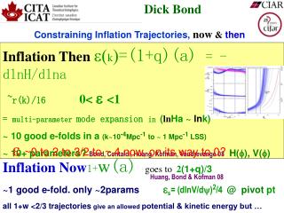
Dick Bond
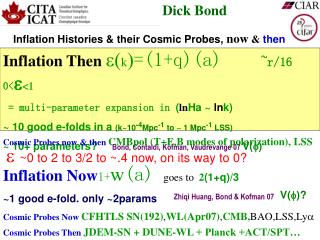
Dick Bond. Inflation & its Cosmic Probes, now & then. Cosmic Probes CMB, CMBpol (E,B modes of polarization) B from tensor: Bicep, Planck, Spider, Spud, Ebex, Quiet, Pappa, Clover, …, Bpol CFHTLS SN(192) , WL(Apr07) , JDEM/DUNE BAO, LSS,Ly a.


Dick Bond
E N D
Presentation Transcript
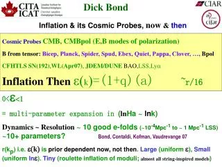
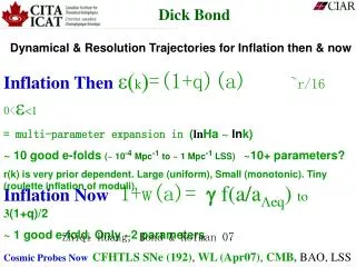
Dick Bond Inflation & its Cosmic Probes, now&then Cosmic Probes CMB, CMBpol (E,B modes of polarization) B from tensor: Bicep, Planck, Spider, Spud, Ebex, Quiet, Pappa, Clover, …, Bpol CFHTLS SN(192),WL(Apr07), JDEM/DUNE BAO,LSS,Lya Inflation Thenk=(1+q)(a) ~r/160< = multi-parameter expansion in (lnHa ~ lnk) Dynamics ~ Resolution~ 10 good e-folds (~10-4Mpc-1 to ~ 1 Mpc-1 LSS) ~10+ parameters? Bond, Contaldi, Kofman, Vaudrevange 07 r(kp) i.e. k is prior dependent now, not then. Large (uniform ), Small (uniform ln). Tiny (roulette inflation of moduli; almost all string-inspired models) KKLMMT etc, Quevedo etal,Bond, Kofman, Prokushkin, Vaudrevange 07, Kallosh and Linde 07 General argument: if the inflaton < the Planck mass, then r < .007 (Lyth96 bound)
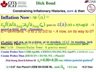
Dick Bond Inflation & its Cosmic Probes, now&then Inflation Now1+w(a)= esf(a/aeq;as/aeq;zs)goes to(a)x3/2 = 3(1+q)/2 ~1 good e-fold. only ~2params Zhiqi Huang, Bond & Kofman 07es=0.0+-0.25 now, late-inflaton (potential gradient)2 to +-0.07 then Planck1+JDEM SN+DUNE WL, weak as < 0.3 now <0.21 then (late-inflaton mass is < Planck mass, but not by a lot) Cosmic Probes NowCFHTLS SN(192),WL(Apr07),CMB,BAO,LSS,Lya Cosmic Probes Then JDEM-SN + DUNE-WL + Planck1
CMB/LSS Phenomenology • Dalal • Dore • Kesden • MacTavish • Pfrommer • Shirokov • CITA/CIfAR there • Mivelle-Deschenes (IAS) • Pogosyan (U of Alberta) • Myers (NRAO) • Holder (McGill) • Hoekstra (UVictoria) • van Waerbeke (UBC) • CITA/CIfAR here • Bond • Contaldi • Lewis • Sievers • Pen • McDonald • Majumdar • Nolta • Iliev • Kofman • Vaudrevange • Huang • UofT here • Netterfield • Carlberg • Yee • & Exptal/Analysis/Phenomenology Teams here & there • Boomerang03 (98) • Cosmic Background Imager1/2 • Acbar07 • WMAP (Nolta, Dore) • CFHTLS – WeakLens • CFHTLS - Supernovae • RCS2 (RCS1; Virmos-Descart) Parameter data now:CMBall_pol SDSS P(k), BAO, 2dF P(k) Weak lens (Virmos/RCS1, CFHTLS, RCS2) ~100sqdeg Benjamin etal. aph/0703570v1 Lya forest (SDSS) SN1a “gold”(192,15 z>1) CFHTLS then:ACT (SZ),Spider, Planck, 21(1+z)cm GMRT,SKA Prokushkin
Dick Bond Inflation & its Cosmic Probes, now&then Inflation now Dynamical background late-inflaton-field trajectories imprint luminosity distance, angular diameter distance, volume growth, growth rate of density fluctuations Prior late-inflaton primordial fluctuation information is largely lost because tiny mass (field sound speed=c?) late-inflaton may have an imprint on other fields? New late-inflaton fluctuating field power is tiny
w-trajectories for V(f):pNGB example e.g.sorbo et07 For a given quintessence potential V(f), we set the “initial conditions” at z=0 and evolve backward in time. w-trajectories for Ωm(z=0) = 0.27 and (V’/V)2/(16πG)(z=0) = 0.25, the 1-sigma limit, varying the initial kinetic energy w0 = w(z=0) Dashed lines are our first 2-param approximation using an a-averaged es= (V’/V)2/(16πG) and c2 -fitted as. Wild rise solutions Slow-to-medium-roll solutions Complicated scenarios: roll-up then roll-down
Approximating Quintessence for Phenomenology 1+w=2sin2 Zhiqi Huang, Bond & Kofman 07 + Friedmann Equations + DM+B Include a w<-1 phantom field, via a negative kinetic energy term 1+w=-2sinh2
slow-to-moderate roll conditions 1+w< 0.3 (for 0<z<10) gives a 2-parameter model (as and es): Early-Exit Scenario: scaling regime info is lost by Hubble damping, i.e.small as CMB+SN+LSS+WL+Lya 1+w< 0.2 (for 0<z<10) and gives a 1-parameter model (as<<1):
Some Models • Cosmological Constant (w=-1) • Quintessence (-1≤w≤1) • Phantom field (w≤-1) • Tachyon fields (-1 ≤ w ≤ 0) • K-essence (no prior on w) w(a)=w0+wa(1-a) Uses latest April’07 SNe, BAO, WL, LSS, CMB, Lya data effective constraint eq.
cf. SNLS+HST+ESSENCE = 192 "Gold" SN illustrates the near-degeneracies of the contour plot
Higher Chebyshev expansion is not useful: data cannot determine >2 EOS parameters9 & 40 into Parameter eigenmodesDETF Albrecht etal06, Crittenden etal06, hbk07 piecewise parameterization 4,9,40 z-modes of w(z) 9 4 s1=0.12 s2=0.32 s3=0.63 40 Data used 07.04: CMB+SN+WL +LSS+Lya
Measuring constant w (SNe+CMB+WL+LSS) 1+w = 0.02 +/- 0.05
Measuring es(SNe+CMB+WL+LSS+Lya) Modified CosmoMC with Weak Lensing and time-varying w models
45 low-z SN + ESSENCE SN + SNLS 1st year SN+ Riess high-z SN, all fit with MLCS SNLS+HST = 182 "Gold" SN SNLS+HST+ESSENCE = 192 "Gold" SN SNLS1 = 117 SN (~50 are low-z)
estrajectoriesareslowly varying: why the fits are good Dynamical ew= (1+w)(a)/f(a) cf. shape eV= (V’/V)2 (a) /(16πG) es= evuniformly averaged over 0<z<2 in a.
3-parameter parameterization next order corrections: Wm (a) (depends on es redefines aeq) ev = es (a) (adds newzs parameter) enforce asymptotic kinetic-dominance w=1(add as power suppression) refine the fit to encompass even baroque trajectories. this choice is analytic. The correction on w is only ~ 0.01
3-parameter fitting es &ζs calculated frome trajectory (linear least square) asisc2-fit • Perfectly fits slow-to-moderate roll
Measuring the 3 parameters with current data • Use 3-parameter formula over 0<z<4 & w(z>4)=wh(irrelevant parameter unless large). as<0.3
Comparing 1-2-3-parameter results CMB + SN + WL + LSS +Lya Conclusion: for current data, the multi-parameter complications are largely irrelevant (as<0.3): we cannot reconstruct the quintessence potential we can only measure the slope es
Thawing, freezing or non-monotonic? With freezing prior: With thawing prior: Thawing: 1+w monotonic up as z decreases Freezing: 1+w monotonic down to 0 as z decreases ~15% thaw, 8% freeze, most non-monotonic with flat priors
Forecast: JDEM-SN(2500 hi-z + 500 low-z)+ DUNE-WL(50% sky, gals @z = 0.1-1.1, 35/min2 ) + Planck1yr Beyond Einstein panel: LISA+JDEM es=0.02+0.07-0.06 ESA as<0.21 (95%CL)
Inflation now summary • the data cannot determine more than 2 w-parameters (+ csound?). general higher order Chebyshev expansion in1+was for “inflation-then”=(1+q)is not that useful. Parameter eigenmodesshow what is probed • The w(a)=w0+wa(1-a) phenomenology requires baroque potentials • Philosophy of HBK07:backtrack from now (z=0) all w-trajectories arising from quintessence(es >0) and the phantom equivalent (es <0); use a 3-parameter model to well-approximate even rather baroque w-trajectories. • We ignore constraints on Q-density from photon-decoupling and BBN because further trajectory extrapolation is needed. Can include via a prior on WQ(a) at z_dec and z_bbn • For general slow-to-moderate rolling one needs 2 “dynamical parameters” (as, es) & WQ to describe w to a few % for the not-too-baroque w-trajectories. • asis < 0.3 current data (zs>2.3) to <0.21 (zs>3.7) in Planck1yr-CMB+JDEM-SN+DUNE-WL future In the early-exit scenario, the information stored inasis erased by Hubble friction over the observable range &w can be described by a single parameteres. • a 3rdparamzs, (~des /dlna) is ill-determined now & in aPlanck1yr-CMB+JDEM-SN+DUNE-WL future • To use: given V, compute trajectories, do a-averaged es& test (or simpler es-estimate) • for eachgiven Q-potential, velocity, amp, shape parameters are needed to define a w-trajectory • current observations are well-centered around the cosmological constantes=0.0+-0.25 • in Planck1yr-CMB+JDEM-SN+DUNE-WL futureesto +-0.07 • but cannot reconstruct the quintessence potential, just the slope es& hubble drag info • late-inflaton mass is < Planck mass, but not by a lot • Aside: detailed results depend upon the SN data set used. Best available used here (192 SN), soon CFHT SNLS ~300 SN + ~100 non-CFHTLS. will put all on the same analysis/calibration footing – very important. • Newest CFHTLS Lensing data is important to narrow the range over just CMB and SN
Dick Bond Inflation & its Cosmic Probes, now&then Inflation then Amplitude As, average slope <ns>, slope fluctuations dns = ns -< ns > (running, running of running, …) for scalar (low L to high L CMB ACT/SPT; Epol Quad, SPTpol, Quiet2, Planck) & tensor At, <nt>, dnt = nt-< nt > (low L <100 Planck, Bicep, EBEX, Spider, SPUD, Clover, Bpol) & isocurvature Ais, <nis>, dnis= nis-< nis> power spectra (subdominant) Blind search for structure (not really blind because of prior probabilities/measures) Fluctuation field power spectra related to dynamical background field trajectories Defines a tensor/scalar functional relation between; both to Hubble & inflaton potential
Standard Parameters of Cosmic Structure Formation Period of inflationary expansion, quantum noise metricperturbations r < 0.6 or < 0.28 95% CL Scalar Amplitude Density of Baryonic Matter Spectral index of primordial scalar (compressional) perturbations Spectral index of primordial tensor (Gravity Waves) perturbations Density of non-interacting Dark Matter Cosmological Constant Optical Depth to Last Scattering Surface When did stars reionize the universe? Tensor Amplitude What is the Background curvature of the universe? closed flat open
New Parameters of Cosmic Structure Formation tensor (GW) spectrum use order M Chebyshev expansion in ln k, M-1 parameters amplitude(1), tilt(2), running(3),... scalar spectrum use order N Chebyshev expansion in ln k, N-1 parameters amplitude(1), tilt(2), running(3), … (or N-1 nodal point k-localized values) Dual Chebyshev expansion in ln k: Standard 6 is Cheb=2 Standard 7 is Cheb=2,Cheb=1 Run is Cheb=3 Run & tensor is Cheb=3, Cheb=1 Low order N,M power law but high order Chebyshev is Fourier-like
New Parameters of Cosmic Structure Formation Hubble parameter at inflation at a pivot pt =1+q, the deceleration parameter history order N Chebyshev expansion, N-1 parameters (e.g. nodal point values) (adaptive Chebyshev groups) Fluctuations are from stochastic kicks ~ H/2p superposed on the downward drift at Dlnk=1. Potential trajectory from HJ (SB 90,91):
TheParameters of Cosmic Structure Formation Cosmic Numerology: aph/0611198 – our Acbar paper on the basic 7+; bckv07 WMAP3modified+B03+CBIcombined+Acbar06+LSS (SDSS+2dF) + DASI (incl polarization and CMB weak lensing and tSZ) ns = .958 +- .015 .93 +- .03 @0.05/Mpc run&tensor r=At / As < 0.28 95% CL <.36 CMB+LSS run&tensor dns /dln k = -.060 +- .022 -.038 +- .024 CMB+LSS run&tensor As = 22 +- 2 x 10⁻¹⁰ Wbh2 = .0226 +- .0006 Wch2= .114 +- .005 WL = .73 +.02 - .03 h = .707 +- .021 Wm= .27 + .03 -.02 zreh =11.4 +- 2.5
CMBology Inflation Histories (CMBall+LSS) subdominant phenomena (isocurvature, BSI) Secondary Anisotropies (tSZ, kSZ, reion) Foregrounds CBI, Planck Polarization of the CMB, Gravity Waves (CBI, Boom, Planck, Spider) Non-Gaussianity (Boom, CBI, WMAP) Dark Energy Histories (& CFHTLS-SN+WL) Probing the linear & nonlinear cosmic web
CBI pol to Apr’05@Chile Bicep @SP Quiet2 (1000 HEMTs) @Chile CBI2 to early’08 Acbar to Jan’06, 07f @SP QUaD @SP Quiet1 SCUBA2 Spider (12000 bolometers) 2312 bolometer @LDB APEX SZA JCMT @Hawaii (~400 bolometers) @Chile (Interferometer) @Cal ACT Clover @Chile (3000 bolometers) @Chile Boom03@LDB EBEX@LDB 2017 2004 2006 2008 LMT@Mexico 2005 2007 SPT LHC 2009 Bpol@L2 WMAP@L2to 2009-2013? (1000 bolometers) @South Pole ALMA DASI @SP (Interferometer) @Chile Polarbear (300 bolometers)@Cal CAPMAP Planck08.8 AMI (84 bolometers) HEMTs @L2 GBT
Inflation in the context of ever changing fundamental theory 1980 -inflation Old Inflation New Inflation Chaotic inflation SUGRA inflation Power-law inflation Double Inflation Extended inflation 1990 Hybrid inflation Natural inflation Assisted inflation SUSY F-term inflation SUSY D-term inflation Brane inflation Super-natural Inflation 2000 SUSY P-term inflation K-flation N-flation DBI inflation inflation Warped Brane inflation Tachyon inflation Racetrack inflation Roulette inflation Kahler moduli/axion
Power law (chaotic) potentials V/MP4 ~ l y2n, y=f/MP2-1/2 e=(n/y)2 , e = (n/2) /(NI(k) +n/3), ns-1= - (n+1) / (NI(k) -n/6), nt= - n/ (NI(k) -n/6), n=1, NI~ 60,r = 0.13, ns= .967, nt= -.017 n=2, NI~ 60,r = 0.26, ns= .950, nt= -.034 MP-2= 8pG
PNGB:V/MP4 ~Lred4sin2(y/fred 2-1/2 ) ns~ 1-fred-2 , e = (1-ns)/2 /(exp[(1-ns)NI (k)](1+(1-ns)/6) -1), exponentially suppressed; higherrif lowerNI & 1-ns to match ns=.96, fred~ 5, r~0.032 to match ns= .97, fred~ 5.8, r~0.048 cf.n=1, r = 0.13, ns= .967, nt= -.017 ABFFO93
Moduli/brane distance limitation in stringy inflation. Normalized canonical inflaton Dy < 1 over DN ~ 50, e.g. 2/nbrane1/2BM06 e = (dy /d ln a)2so r = 16e < .007, <<? roulette inflation examples r ~ 10-10 & Dy < .002 possible way out with many fields assisting: N-flation ns= .97, fred~ 5.8, r~0.048, Dy ~13 cf.n=1, r = 0.13, ns= .967, Dy ~10 cf.n=2, r = 0.26, ns= .95, Dy ~16
energy scale of inflation & r V/MP4 ~ Ps r (1-e/3)3/2 V~ (1016Gev)4r/0.1 (1-e/3) roulette inflation examples V~ (few x1013Gev)4 H/MP ~ 10-5 (r/.1)1/2 inflation energy scale cf. the gravitino mass (Kallosh & Linde 07) if a KKLT/largeVCY-likegeneration mechanism 1013Gev (r/.01)1/2 ~ H < m3/2cf. ~Tev
String Theory Landscape& Inflation++ Phenomenology for CMB+LSS Hybrid D3/D7 Potential • D3/anti-D3 branes in a warped geometry • D3/D7 branes • axion/moduli fields ... shrinking holes KKLT, KKLMMT BB04, CQ05, S05, BKPV06 f|| fperp large volume 6D cct Calabi Yau
B-pol simulation:input LCDM (Acbar)+run+uniform tensor r (.002 /Mpc) reconstructed cf. rin esorder 5 log prior esorder 5 uniform prior a very stringent test of the e-trajectory methods: A+
Planck1yr simulation:input LCDM (Acbar)+run+uniform tensor r (.002 /Mpc) reconstructed cf. rin esorder 5 log prior esorder 5 uniform prior
Planck1 simulation:input LCDM (Acbar)+run+uniform tensor PsPtreconstructed cf. input of LCDM with scalar running & r=0.1 esorder 5 log prior esorder 5 uniform prior r=0.144 +- 0.032 r=0.096 +- 0.030
Planck1 simulation:input LCDM (Acbar)+run+uniform tensor PsPtreconstructed cf. input of LCDM with scalar running & r=0.1 esorder 5 uniform prior esorder 5 log prior lnPslnPt(nodal 5 and 5)
Inflation then summary the basic 6 parameter model with no GW allowed fits all of the data OK Usual GW limits come from adding r with a fixed GW spectrum and no consistency criterion (7 params). Adding minimal consistency does not make that much difference (7 params) r (<.28 95%) limit comes from relating high k region of 8 to low k region of GW CL Uniform priors in (k) ~ r(k): with current data, the scalar power downturns ((k) goes up) at low k if there is freedom in the mode expansion to do this. Adds GW to compensate, breaks old r limit. T/S (k) can cross unity. But log prior in drives to low r. a B-pol could break this prior dependence, maybe Planck+Spider. Complexity of trajectories arises in many-moduli string models. Roulette example: 4-cycle complex Kahler moduli in large compact volume Type IIB string theory TINY r ~ 10-10 if the normalized inflaton y < 1 over ~50 e-folds thenr <.007Dy ~10 for power law & PNGB inflaton potentials Prior probabilities on the inflation trajectories are crucial and cannot be decided at this time. Philosophy: be as wide open and least prejudiced as possible Even with low energy inflation, the prospects are good with Spider and even Planck to either detect the GW-induced B-mode of polarization or set a powerful upper limit against nearly uniform acceleration. Both have strong Cdn roles.CMBpol