Dick Bond
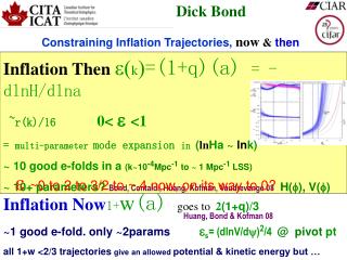
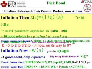
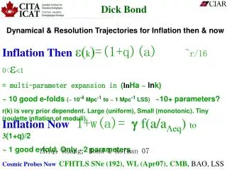
Dynamical & Resolution Trajectories for Inflation then & now. Inflation Then e( k ) =(1+q)(a) ~r/16 0< e <1 = multi-parameter expansion in ( ln Ha ~ ln k) ~ 10 good e-folds (~ 10 -4 Mpc -1 to ~ 1 Mpc -1 LSS) ~10+ parameters?

Dick Bond
E N D
Presentation Transcript
Dynamical & Resolution Trajectories for Inflation then & now Inflation Then e(k)=(1+q)(a) ~r/160<e<1 = multi-parameter expansion in (lnHa ~ lnk) ~ 10 good e-folds (~ 10-4 Mpc-1 to ~ 1 Mpc-1 LSS) ~10+ parameters? r(k) is very prior dependent. Large (uniform), Small (monotonic). Tiny (roulette inflation of moduli). Dick Bond Inflation Now 1+w(a)= gf(a/aLeq)to3(1+q)/2 ~ 1 good e-fold. Only ~2 parameters Zhiqi Huang, Bond & Kofman 07 Cosmic Probes NowCFHTLS SNe (192), WL (Apr07), CMB, BAO, LSS
Some Models • Cosmological Constant (w=-1) • Quintessence (-1≤w≤1) • Phantom field (w≤-1) • Tachyon fields (-1 ≤ w ≤ 0) • K-essence (no prior on w) Uses latest April’07 SNe, BAO, WL, LSS, CMB data Higher Chebyshev expansion is not useful: data cannot determine >2 EOS parameters.e.g., Crittenden etal.06 Parameter eigenmodes effective constraint eq.
Zhiqi Huang, Bond & Kofman 07 Approximating Quintessence for Phenomenology + Friedmann Equations g=λ2
slow-to-moderate roll conditions 1+w< 0.3 (for 0<z<2) and g ~ constgive a 2-parameter model: g=λ2 & aex Early-Exit Scenario: scaling regime info is lost by Hubble damping, i.e.small aex 1+w< 0.2 (for 0<z<10) and g ~ constgive a 1-parameter model:
w-trajectories cf. the 2-parameter model g= (V’/V)2 (a) a-averaged at low z the field exits scaling regime at a~aex
w-trajectories cf. the 1-parameter model ignore aex g= (V’/V)2 (a) a-averaged at low z
Include a w<-1 phantom field, via a negative kinetic energy term φ -> iφ g=λ2< 0
Measuring g=λ2 (SNe+CMB+WL+LSS) Well determined g undetermined aex aex
Measuring g=λ2 (SNe+CMB+WL+LSS) Modified CosmoMC with Weak Lensing and time-varying w models
g-trajectories cf. the 1-parameter model g=(1+w)(a)/f(a) cf. (V’/V)2 (a)
SNLS+HST = 182 "Gold" SN 45 low-z SN + ESSENCE SN + SNLS 1st year SN+ Riess high-z SN, all fit with MLCS SNLS+HST+ESSENCE = 192 "Gold" SN SNLS1 = 117 SN (~50 are low-z)
Inflation now summary • The data cannot determine more than 2 w-parameters (+ csound?). general higher order Chebyshev expansion in 1+w as for “inflation-then” e=(1+q)is not that useful – cf. Roger B & co. • The w(a)=w0+wa(1-a) expansion requires baroque potentials • For general slow-to-moderate rolling one needs 2 “dynamical parameters” (aex,g) to describe w to a few % (cf. for a given Q-potential, IC, amp, shape to define a w-trajectory) • In the early-exit scenario, the information stored in aex is erased by Hubble friction, w can be described by a single parameter g. aex is not determined by the current data • phantom (g <0), cosmological constant (g=0), and quintessence (g >0) are all allowed with current observations g =0.0+-0.5 • Aside: detailed results depend upon the SN data set used. Best available used here (192 SN), but this summer CFHT SNLS will deliver ~300 SN to add to the ~100 non-CFHTLS and will put all on the same analysis footing – very important. • Lensing data is important to narrow the range over just CMB and SN
Inflation then summary the basic 6 parameter model with no GW allowed fits all of the data OK Usual GW limits come from adding r with a fixed GW spectrum and no consistency criterion (7 params). Adding minimal consistency does not make that much difference (7 params) r (<.28 95%) limit come from relating high k region of s8 to low k region of GW CL Uniform priors in e(k) ~ r(k): the scalar power downturns (e(k) goes up) at low L if there is freedom in the mode expansion to do this. Adds GW to compensate, breaks old r limit. T/S (k) can cross unity. But monotonic prior in e drives to low energy inflation and low r. Complexity of trajectories could come out of many-moduli string models. Roulette example: 4-cycle complex Kahler moduli in Type IIB string theory TINY r ~ 10-10a general argument that the normalized inflaton cannot change by more than unity over ~50 e-folds givesr <10-3 Prior probabilities on the inflation trajectories are crucial and cannot be decided at this time. Philosophy: be as wide open and least prejudiced as possible Even with low energy inflation, the prospects are good with Spider and even Planck to either detect the GW-induced B-mode of polarization or set a powerful upper limit against nearly uniform acceleration. Both have strong Cdn roles.