Download
1 / 37
370 likes | 396 Views
This paper presents a hybrid numerical method for non-stationary continuum mechanics, using moving adaptive grids, equilibrated viscosity scheme, and overlapping grids. The method is advantageous for problems in moving regions of complex geometry.

E N D
HYBRID NUMERICAL METHOD FOR NON-STATIONARY CONTINUUM MECHANICS N.G. Burago1,3, I.S. Nikitin2,3 1IPMechRAS,2ICADRAS, 3Bauman MSTU Volodarka - 2015
Under consideration: Problems of Continuum Mechanics in Moving Regions of Complex Geometry Advantage of three method components: 1. Moving Adaptive Grids2. Equilibrated Viscosity Scheme3. Overlapping Grids
Types of Grid Adaption1) Region boundaries of complex shape2) Minimization of approximation errors (min|hdy/dx| )
Basement: Non-linear thermo-elasticity equations for adaptive grid generation N.G.Bourago and S.A.Ivanenko, Application of nonlinear elasticity to the problem of adaptive grid generation // Proc. Russian Conf. on Applied Geometry, Grid Generation and High Performance Computing, Computing Center of RAS, Moscow, 2004, June 28 - July 1. P. 107-118.
Governing variational equation Cell shape control parameter Cell compressibility parameter Thermal expantion (monitor function, “anti-temperature”)
Method for grid equation - stabilization method Algorithm: two-layered explicit scheme of stabilization which provides equilibrium (by norm) of members with L and f Details: ipmnet.ru/~burago
2. Equilibrated Viscosity Scheme(Variant of stabilized Petrov-Galerkin scheme)
Variational Equations for Fluid Dynamics Уравнения для задач механики жидкости и газа Equations for Solid Mechanics are analogical Уравнения для твердых деформируемых сред аналогичны
Simplifiedexplicitscheme SUPG FEM1(variant ofstabilizedPetrov-Galerkin method) то если иначе 1Brooks A.N., Hughes T.J.R. Streamline Upwind Petrov-Galerkin formulations for convection dominated flows // Computer Methods in Applied Mechanics and Engineering. 32. (1982) pp. 199-259. Artifitial diffusion“equilibrates”by norminviscous fluxes Inviscous fluxes = convective terms + conservative parts of fluxes Simplification: used FEM scheme is analogical to centraldifference scheme
Коррекция физической вязкости по А.А.Самарскому (“экспоненциальная подгонка”) Corrected (by A.A.Samarsky) physical viscosity (“exponential correction scheme”) Courant–Friedrichs–Lewy stability condition Условие устойчивости (Курант-Фридрихс-Леви) Doolan E.P., Miller J.J.H., Schilders W.H.A. Uniform numerical methods for problems with initial and boudary layers. BOOLE PRESS. Dublin. 1980. Physical viscosity is decreasing with growth of artificial viscosity
Briefresume of numerical method. Galerkin formulation. Simplex finite elements.Adaptivemoving grid. All major unknowns in nodes. FEManalogy of central difference schemes in space. Explicit scheme for compressible media: Variant of stabilized Petrov-Galerkin scheme Explicit (convection fluxes) - implicit (concervative and dissipative fluxes) scheme for incompressible or low Mach flows Exponential correction of physical viscosity. Adaption: separated stage at the end of each time step
Ideal gas flow in channel with a step: М=3; g=1.4; t = 0; 0.5; Adapted grid
Ideal gas flow in channel with a step: М=3; g=1.4; t = 1.0; 2.0; Adapted grid
Ideal gas flow in channel with a step: М=3; g=1.4; t = 3.0; 4.0; Adapted grid
Ideal gas flow in channel with a step: М=3; g=1.4; t = 4.0; Isolines of density; Adaption using as monitor function
Adaptive grids for supersonic flows inchannels with obstacles
Adaptive grid for turbine blade forming process. maintenance of uniform distribution of nodes
3. Overlapping grids for calculation problems with complex geometry
Overlapping grids – what for?For example:Supersonic flows over several obstacles Grid with triangular holeMain and overlapping grids
Overlapping or Chimera grids + Main bordering grid Additional overlapping grids Calculation is carried out by steps according to the explicit scheme or by iterations according to the implicit scheme separately on the main grid and on the overlapping grids, thus after each step (iteration) by means of interpolation the exchange of data between grids in an overlapping zone is carried out.
Simpified overlapping grid method Target: simple solution of complex geometry problem + Main bordering grid Additional overlapping grids The overlapping grids are used only for complex boundary description and for boundary conditions on the main grid ========================== Instead of overlapping grids here the overlapping areas defined by the set of conditions may be used
Part of solution region near overlapping grid (an obstacle)(velocities att=0)
Part of solution region near overlapping grid (an obstacle). Main grid is adaptive and moving (velocities att=0.1)
Part of solution region near overlapping grid (an obstacle). Main grid is adaptive and moving (velocities att=0.2)
Part of solution region near overlapping grid (an obstacle). Main grid is adaptive and moving (velocities att=0.3)
Part of solution region near overlapping grid (an obstacle).Isolines of vertical velocity att=0.
Part of solution region near overlapping grid (an obstacle).Isolines of vertical velocity att=0.1
Part of solution region near overlapping grid (an obstacle).Isolines of vertical velocity att=0.2
Part of solution region near overlapping grid (an obstacle).Isolines of vertical velocity att=0.3
Part of solution region near overlapping grid (an obstacle).Isolines of local Mach number att=0.45
Whole solution region with two overlapping grids (an obstacles).Isolines of local Mach number att=0.45
Whole solution region with two overlapping grids (obstacles).Isolines of local Mach number att=7.0
Whole solution region with two overlapping grids (obstacles).Isolines of major unknown functions att=7.0
Conclusions. Implementationis rather easy possible as an addition to any normal gas dynamic code, capable to solve problems in rectangular or brick like solution region. It just needs to add separated blocks for setting overlapping areas and at the end of each step (iteration) it needs to provide correction of solution on overlapping parts of major gridin order to satisfyboundary conditions. Advantages.Simplified overlapping grid method allows easily take into account complex geometry and boundary conditions. Equilibrated viscosity scheme and elastic grid adaptation technique provide together high accuracy of solution and robustness. There is no dependence of governing parameters of scheme on type of problem, the number of parameters is small and each has clear meaning. Drawbacks.To provide necessary accuracy of solution rather high performance computers are required. Therefore personal computers are effective and give good accuracy only for 2D unsteady problems. For мore detailed information see WEB: http://www.ipmnet.ru/~burago