Download
1 / 31
310 likes | 347 Views
This study delves into the role of anti-parallel merging and component reconnection in magnetospheric dynamics using global MHD simulations. Exploring the fast reconnection rate in kinetic/two-fluid models within MHD simulations, it investigates the impact of IMF clock angle and analyzes possible reconnection sites like sub-solar flow stagnation points and magnetically neutral points. The research examines the role of high-speed flows at the flanks and the behavior at magneto-neutral points, flux rope formation, and component reconnection dynamics at various IMF orientations using detailed numerical analysis and simulations.

E N D
Anti-Parallel Merging and Component Reconnection: Role in Magnetospheric Dynamics M.M Kuznetsova, M. Hesse, L. Rastaetter NASA/GSFC T. I. Gombosi University of Michigan
I. How to reproduce fast reconnection rate of kinetic/two-fluid models in MHD simulations? Small- meso-scale simulations with nongyrotropic corrections Numerical viscosity vs. uniform resistivity. II. How global MHD models describe dayside magnetic reconnection? What is the impact of the IMF clock angle ?
Possible Reconnection Sites. Sub-Solar Flow Stagnation Point: V = 0 Component Reconnection for By 0 ? Magnetically Neutral Points (cusp region, flanks): B = 0 What is the Role of High Speed Flows at Flanks? Reconnection Line Extended Over the Entire Dayside Magnetopause
How global MHD models describe dayside magnetic reconnection? Steady-state or impulsive reconnection (FTEs, flux ropes ?) Role of velocity sheer at neutral points (K-H instability ?)
Model Global MHD simulation model: BATSRUS, University of Michigan BATSRUS uses an adaptive grid composed of rectangular blocks arranged in varying degrees of spatial refinement levels. Grid Simulation Box -255 Re < X < 33 Re |Y|, |Z| < 96 Re Medium Resolution Runs 1/4 Re: Dayside Magnetosphere + Central Plasma Sheet High Resolution Runs 1/16 Re: Dayside Magnetopause Including Flanks
Solar Wind Parameters: N = 2 cm –3 , T = 20,000 Ko , Vx = 300 km/s, |B| = 5 nT Simulation Startup: 0:00 – 2:00 - StartupBz = - 5nT 2:00 – 4:00 – Northward IMF Bz = 5 nT IMF Turning From Northward Orientation (θ= 0) to IMF Clock angles 105 < θ < 180: 4:00 – 4:05 Run 1: θ = 180 Run 2: θ = 135 Run 3: θ= 120 Run 4: θ= 105 Fixed IMF 4:05 – 7:00
Time Interval of Interest 4:00 – 6:00(0 – 120 min) After IMF Turning 04:00 Prior to Night-Side Reconnection Onset Rate of dayside reconnection can be estimated as the rate of the polar cap growth
Component Reconnection at Sub-Solar Stagnation Point for Large By (θ = 105) X = 13.7 Re Y = 0 Z = 0
What is going on at magnetically neutral points at the flanks? What is the role of high speed flows? θ= 135 X = 1.5 Re Y = 15 Re Z = 6 Re
Open Magnetic Flux Increase = Total Reconnected Flux Growth θ= 180 θ= 135 Wb ] θ= 120 θ= 105 [10 9 Flux time (min )
Ψlocal= L =Ψtotal/ Ψlocal Emax dt * 2 Re L - Effective Lengthof Reconnection Line θ = 180 θ = 135 θ = 120 θ = 105 L [Re] L ~ 2 * R R = 13.7 Re R - distance to the sub-solar point time ( min )
θ = 180 Z = 0 Y = 0
Y = 0 Z = 0 θ = 180
Flux Rope Formation at Sub-Solar Stagnation Region for 120 < < 135?
Flux Rope Formation θ = 120 Pressure
Flux Rope Formation θ = 120 Magnetic Field By Density
θ = 120 Flux Rope Formation
t = 80 min Flux Rope Evolution = 120
High resolution global MHD simulations demonstrated flux ropes (FTEs) generation by intermittent component reconnection. • We show that FTEs are flux ropes of approximate size 1-2 Re with strong core magnetic field imbedded in the magnetopause. • FTE bulge is larger on the magnetosheath side than on the magnetosphere side. The flow around the flux rope is largest at the magnetosphere side. • The plasma pressure pattern within the flux rope exhibit a ring-shaped structure surrounding a central depression. • Traveling density depletion.
Anatomy of flux transfer event seen by Cluster Sonnerup, Hasegawa, and Paschmann, Geophys. Res. Letters, L11803, 2004 Pressure Magnetic Field
Summary High resolution global MHD simulations demonstrated sub-solar component reconnection for IMF clock angles 105 <θ< 180. The rate of reconnection flux loading vary no more than 5-10 % for different IMF orientations in range of IMF Clock angles 105 < θ < 180. Flux budget analysis indicate that magnetic field is reconnection along extended region comparable with magnetopause scale. High resolution simulation demonstrated instability of extended reconnection region and formation of plasmoids and flux ropes. K-H instability is developing close to neutral points in region of fast flows at magnetopause flanks.
Reconnected Flux at Sub-Solar Region |Y| < 1 Re E0 E2 E1 Ψ= E0 dt * 2 Re
Open Magnetic Flux Increase (Resolution 1/16 Re) Theta = 180 Wb ] Theta = 135 [10 9 Theta = 120 Flux Theta = 105 time (min )
Reconnected FluxΨat Subsolar Region |Y| < 1 Re Total Reconnected Flux med resolution (1/4 Re) high resolution (1/16 Re) (1/4 Re) (1/16 Re) 0.6 0.5 0.4 0.3 0.2 0.1 0.0 0.6 0.5 0.4 0.3 0.2 0.1 0.0 θ = 180 θ = 135 Wb ] Wb ] [10 9 [10 9 Flux Flux 0 20 40 60 80 100 120 0 20 40 60 80 100 120 time (min) time (min) 0.6 0.5 0.4 0.3 0.2 0.1 0.0 0.6 0.5 0.4 0.3 0.2 0.1 0.0 θ= 120 θ= 105 Wb ] Wb ] [10 9 [10 9 Flux Flux 0 20 40 60 80 100 120 0 20 40 60 80 100 120 time (min) time (min)
θ = 180 θ = 135
t = 84 min Flux Rope Evolution = 120