Download
1 / 65
700 likes | 895 Views
Efficient Logistic Regression with Stochastic Gradient Descent: The Continuing Saga. William Cohen. Outline. SGD review The “hash trick” the idea an experiment Other randomized algorithms Bloom filters Locality sensitive hashing. Learning as optimization: general procedure for SGD.

E N D
Efficient Logistic Regression with Stochastic Gradient Descent:The Continuing Saga William Cohen
Outline • SGD review • The “hash trick” • the idea • an experiment • Other randomized algorithms • Bloom filters • Locality sensitive hashing
Learning as optimization: general procedure for SGD • Goal: Learn the parameter θ of … • Dataset: D={x1,…,xn} • or maybe D={(x1,y1)…,(xn, yn)} • Write down Pr(D|θ) as a function of θ • Big-data problem: we don’t want to load all the data D into memory, and the gradient depends on all the data • Solution: • pick a small subset of examples B<<D • approximate the gradient using them • “on average” this is the right direction • take a step in that direction • repeat…. B = one example is a very popular choice
Learning as optimization for logistic regression • Goal: Learn the parameter θ of a classifier • Which classifier? • We’ve seen y = sign(x . w) but sign is not continuous… • Convenient alternative: replace sign with the logistic function
Learning as optimization for logistic regression • Goal: Learn the parameter w of the classifier • Probability of a single example (y,x) would be • Or with logs:
And the gradient is… • Key computational point: • if xj=0 then the gradient of wjis zero • so when processing an example you only need to update weights for the non-zero features of an example.
Learning as optimization for logistic regression • Final algorithm: -- do this in random order
Learning as optimization for logistic regression • Goal: Learn the parameter θ of a classifier • Which classifier? • We’ve seen y = sign(x . w) but sign is not continuous… • Convenient alternative: replace sign with the logistic function • Practical problem: this overfits badly with sparse features • e.g., if wjis only in positive examples, its gradient is always positive !
Regularized logistic regression • Replace LCL • with LCL + penalty for large weights, eg • So: • becomes:
Regularized logistic regression • Replace LCL • with LCL + penalty for large weights, eg • So the update for wj becomes: • Or
Learning as optimization for regularized logistic regression • Algorithm: • Time goes from O(nT) to O(nmT) where • n = number of non-zero entries, • m = number of features, • T = number of passes over data
Learning as optimization for regularized logistic regression • Final algorithm: • Initialize hashtableW • For each iteration t=1,…T • For each example (xi,yi) • pi = … • For each feature W[j] • W[j] = W[j] - λ2μW[j] • If xij>0 then • W[j] =W[j] + λ(yi- pi)xj
Learning as optimization for regularized logistic regression • Final algorithm: • Initialize hashtableW • For each iteration t=1,…T • For each example (xi,yi) • pi = … • For each feature W[j] • W[j] *= (1 - λ2μ) • If xij>0 then • W[j] =W[j] + λ(yi- pi)xj
Learning as optimization for regularized logistic regression • Final algorithm: • Initialize hashtablesW, A andset k=0 • For each iteration t=1,…T • For each example (xi,yi) • pi = … ; k++ • For each feature W[j] • If xij>0 then • W[j] *= (1 - λ2μ)k-A[j] • W[j] =W[j] + λ(yi- pi)xj • A[j] = k k-A[j] is number of examples seen since the last time we did an x>0 update on W[j]
Learning as optimization for regularized logistic regression • Final algorithm: • Initialize hashtablesW, A andset k=0 • For each iteration t=1,…T • For each example (xi,yi) • pi = … ; k++ • For each feature W[j] • If xij>0 then • W[j] *= (1 - λ2μ)k-A[j] • W[j] =W[j] + λ(yi- pi)xj • A[j] = k • Time goes from O(nmT) back to to O(nT) where • n = number of non-zero entries, • m = number of features, • T = number of passes over data • memory use doubles (m 2m)
Fixes and optimizations • This is the basic idea but • we need to apply “weight decay” to features in an example before we compute the prediction • we need to apply “weight decay” before we save the learned classifier • my suggestion: • an abstraction for a logistic regression classifier
A possible SGD implementation class SGDLogistic Regression { /** Predict using current weights **/ double predict(Map features); /** Apply weight decay to a single feature and record when in A[ ]**/ void regularize(string feature, intcurrentK); /** Regularize all features then save to disk **/ void save(stringfileName,intcurrentK); /** Load a saved classifier **/ static SGDClassifierload(StringfileName); /** Train on one example **/ void train1(Map features, double trueLabel, intk) { // regularize each feature // predict and apply update } } // main ‘train’ program assumes a stream of randomly-ordered examples and outputs classifier to disk; main ‘test’ program prints predictions for each test case in input.
A possible SGD implementation class SGDLogistic Regression { … } // main ‘train’ program assumes a stream of randomly-ordered examples and outputs classifier to disk; main ‘test’ program prints predictions for each test case in input. <100 lines (in python) Other mains: • A “shuffler:” • stream thru a training file T times and output instances • output is randomly ordered, as much as possible, given a buffer of size B • Something to collect predictions + true labels and produce error rates, etc.
A possible SGD implementation • Parameter settings: • W[j] *= (1 - λ2μ)k-A[j] • W[j] =W[j] + λ(yi - pi)xj • I didn’t tune especially but used • μ=0.1 • λ=η* E-2 where Eis “epoch”, η=½ • epoch: number of times you’ve iterated over the dataset, starting at E=1
Pop quiz • Most of the weights in a classifier are • small and not important
How can we exploit this? • One idea: combine uncommon words together randomly • Examples: • replace all occurrances of “humanitarianism” or “biopsy” with “humanitarianismOrBiopsy” • replace all occurrances of “schizoid” or “duchy” with “schizoidOrDuchy” • replace all occurrances of “gynecologist” or “constrictor” with “gynecologistOrConstrictor” • … • For Naïve Bayes this breaks independence assumptions • it’s not obviously a problem for logistic regression, though • I could combine • two low-weight words (won’t matter much) • a low-weight and a high-weight word (won’t matter much) • two high-weight words (not very likely to happen) • How much of this can I get away with? • certainly a little • is it enough to make a difference? how much memory does it save?
How can we exploit this? • Another observation: • the values in my hash table are weights • the keys in my hash table are strings for the feature names • We need them to avoid collisions • But maybe we don’t care about collisions? • Allowing “schizoid” & “duchy” to collide is equivalent to replacing all occurrences of “schizoid” or “duchy” with “schizoidOrDuchy”
Learning as optimization for regularized logistic regression • Algorithm: • Initialize hashtablesW, A andset k=0 • For each iteration t=1,…T • For each example (xi,yi) • pi = … ; k++ • For each feature j: xij>0: • W[j] *= (1 - λ2μ)k-A[j] • W[j] =W[j] + λ(yi- pi)xj • A[j] = k
Learning as optimization for regularized logistic regression • Algorithm: • Initialize arrays W, A of size R andset k=0 • For each iteration t=1,…T • For each example (xi,yi) • Let Vbe hash table so that • pi = … ; k++ • For each hash value h: V[h]>0: • W[h] *= (1 - λ2μ)k-A[j] • W[h] =W[h] + λ(yi- pi)V[h] • A[j] = k
Learning as optimization for regularized logistic regression • Algorithm: • Initialize arrays W, A of size R andset k=0 • For each iteration t=1,…T • For each example (xi,yi) • Let Vbe hash table so that • pi = … ; k++ • For each hash value h: V[h]>0: • W[h] *= (1 - λ2μ)k-A[j] • W[h] =W[h] + λ(yi- pi)V[h] • A[j] = k ???
Learning as optimization for regularized logistic regression • Algorithm: • Initialize arrays W, A of size R andset k=0 • For each iteration t=1,…T • For each example (xi,yi) • Let Vbe hash table so that • pi = … ; k++ ???
An interesting example • Spam filtering for Yahoo mail • Lots of examplesand lots of users • Two options: • one filter for everyone—but users disagree • one filter for each user—but some users are lazy and don’t label anything • Third option: • classify (msg,user) pairs • features of message i are words wi,1,…,wi,ki • feature of user is his/her id u • features of pair are: wi,1,…,wi,ki and uwi,1,…,uwi,ki • based on an idea by Hal Daumé, used for transfer learning
An example • E.g., this email to wcohen • features: • dear, madam, sir,…. investment, broker,…, wcohendear, wcohenmadam, wcohen,…, • idea: the learner will figure out how to personalize my spam filter by using the wcohenX features
An example Compute personalized features and multiple hashes on-the-fly: a great opportunity to use several processors and speed up i/o
Experiments • 3.2M emails • 40M tokens • 430k users • 16T unique features – after personalization
An example 2^26 entries = 1 Gb @ 8bytes/weight
Some details Slightly different hash to avoid systematic bias mis the number of buckets you hash into (R in my discussion)
Some details Slightly different hash to avoid systematic bias mis the number of buckets you hash into (R in my discussion)
Some details I.e. – a hashed vector is probably close to the original vector
Some details I.e. the inner products between x and x’ are probably not changed too much by the hash function: a classifier will probably still work
The hash kernel: implementation • One problem: debugging is harder • Features are no longer meaningful • There’s a new way to ruin a classifier • Change the hash function • You can separately compute the set of all words that hash to hand guess what features mean • Build an inverted index hw1,w2,…,
A variant of feature hashing • Hash each feature multiple times with different hash functions • Now, each w has k chances to not collide with another useful w’ • An easy way to get multiple hash functions • Generate some random strings s1,…,sL • Let the k-th hash function for w be the ordinary hash of concatenation wsk
A variant of feature hashing • Why would this work? • Claim: with 100,000 features and 100,000,000 buckets: • k=1 Pr(any duplication) ≈1 • k=2 Pr(any duplication)≈0.4 • k=3 Pr(any duplication)≈0.01
Experiments Shi et al, JMLR 2009 http://jmlr.csail.mit.edu/papers/v10/shi09a.html • RCV1 dataset • Use hash kernels with TF-approx-IDF representation • TF and IDF done at level of hashed features, not words • IDF is approximated from subset of data • Not sure of value of “c” or data subset
Bloom filters • Interface to a Bloom filter • BloomFilter(intmaxSize, double p); • void bf.add(Strings); // insert s • boolbd.contains(Strings); • // If s was added return true; • // else with probability at least 1-p return false; • // else with probability at most p return true; • I.e., a noisy “set” where you can test membership (and that’s it) • Hash table: constant time and storage
Bloom filters • Another implementation • Allocate M bits, bit[0]…,bit[1-M] • Pick K hash functions hash(1,s),hash(2,s),…. • E.g: hash(s,i) = hash(s+ randomString[i]) • To add string s: • For i=1 to k, set bit[hash(i,s)] = 1 • To check contains(s): • For i=1 to k, test bit[hash(i,s)] • Return “true” if they’re all set; otherwise, return “false” • We’ll discuss how to set M and K soon, but for now: • Let M = 1.5*maxSize// less than two bits per item! • Let K = 2*log(1/p) // about right with this M
Bloom filters • Analysis: • Assume hash(i,s) is a random function • Look at Pr(bit j is unset after n add’s): • … and Pr(collision): • …. fix m and n and minimize k: k =
Bloom filters • Analysis: • Assume hash(i,s) is a random function • Look at Pr(bit j is unset after n add’s): • … and Pr(collision): • …. fix m and n, you can minimize k: p = k =