Download
1 / 16
160 likes | 681 Views
ANALYSIS AND FORECASTING OF LUMPY DEMAND: ALTERNATIVE APPROACHES. Somnath Mukhopadhyay Rafael S. Gutierrez Adriano O. Solis The University of Texas at El Paso. Introduction. Lumpy demand pattern Well-referenced time-series models Neural Network model Research Method Results

E N D
ANALYSIS AND FORECASTING OF LUMPY DEMAND: ALTERNATIVE APPROACHES Somnath Mukhopadhyay Rafael S. Gutierrez Adriano O. Solis The University of Texas at El Paso
Introduction • Lumpy demand pattern • Well-referenced time-series models • Neural Network model • Research Method • Results • Conclusion and Future Research
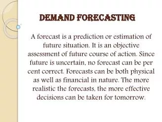
Lumpy Demand Pattern • Defined as a demand with great differences between each period’s requirements and with a great number of periods with zero requests” (Ghobbar and Friend, 2003), and is specified by ADI > 1.32 (where ADI refers to average inter-demand interval) and CV2 > 0.49. • Significant past research on forecasting lumpy demand (Ghobbar, A.A. and C.H. Friend, 2002, 2003; Syntetos, A.A. and J.E. Boylan, 2001,2005; Syntetos, A.A., J.E. Boylan, and J.D. Croston, 2005 )
Lumpy Demand FactorsM is the number of nonzero demand observations in the series and N is the number of intervals with consecutive zero demandsWe identify two factors that might impact relative performance of alternative forecasting methods: (1) the sizes S of nonzero demand transactions and (2) the lengths I of intervals of consecutive zero demands (between nonzero demand transactions)
Time-series Forecasting Model • Ghobbar and Friend (2003) refer to the single exponential smoothing (SES) method as the “standard” method, in practice, for forecasting intermittent demand. • Evaluation of SES as a forecasting technique is fairly common in the literature on lumpy demand forecasting (among many others, Ghobbar and Friend, 2003; Levén and Segerstedt, 2004; Willemain et al., 2004; Syntetos and Boylan, 2005; Regattieri et al., 2005) • Croston (1972) observed that, when demand is intermittent, single exponential smoothing generally leads to inappropriate stock levels in inventory control systems
Modified Croston Method • Croston(1972) proposed a new method of forecasting intermittent demand, involving both the average size of nonzero demand occurrences and the average interval between consecutive occurrences • An error in Croston’s mathematical derivation of expected demand size was reported by Syntetos and Boylan (2001) • Syntetos and Boylan (2005) and Syntetos et al. (2005) introduced a correction factor of (1-alpha/2) to arrive at a modified demand forecast
Neural Network Models • Connectionist theory of pattern seeking in data • Functional relationship determined by going through the data • Flexible enough to respond to sudden changes in data • No assumption of parametric distribution required
Research Method • Analyze Lumpiness Factor • Run ES, MC, and NN models • Compare model performances • Conclude
Method (contd.) Model Parameters • We used the same four smoothing constant values of 0.05, 0.10, 0.15, and 0.20 used by Syntetos and Boylan (2005) in single exponential smoothing, Croston’s method, and the modified Croston • We used 3-layered MLP, n (# of hidden units) = 3 • Network training algorithm back-propagation (BP) • We used learning rate = 0.1 and momentum factor = 0.9
Data We used real lumpy demand data. Each of the 24 time series in our data set consists of 967 observations. We used the first 624 observations of each series to train and validate the models (the training sample). We then tested, at each of the four values of alpha, the four forecasting models under consideration on the final 343 observations (the test sample).
Conclusion • Simple NN models are generally superior to MC and ES in forecasting lumpy demand • NN models are flexible in creating rich prediction surfaces • NN performance is not superior for high AADSmean of series 24
Future Research • Analyze series 24 data further • Use other error statistics like PBEST, RGRMSE • Try different NN models to further improve the forecasting performance • Generating hybrid forecasting models by combining NN and other methods