Download

1 / 18
180 likes | 360 Views
Sect. 6.6: Damped, Driven Pendulum. Consider a plane pendulum subject to an an applied torque N & subject to damping by the viscosity η of the medium (say, air) in which it swings . Mass m . See figure: The angle of swing is allowed in the entire range: - π π

E N D
Sect. 6.6: Damped, Driven Pendulum • Consider a plane pendulum subject to an anappliedtorque N & subject to damping by the viscosity η of the medium (say, air) in which it swings. Mass m. See figure: The angle of swing is allowed in the entire range: -π π The usual assumption of a massless rod. Length = R
First,a simple pendulum, no applied torque.Newton’s 2nd Law or Lagrange’s equations give the equation of motion: Ngrav = Iα = I(d2/dt2), I = mR2 Ngrav = - mgR sin mR2(d2/dt2) + mgRsin = 0 (1) NOTE:The motion is clearly NOTsimple harmonic! • For small angles sin & (1) becomes: mR2(d2/dt2) + mgR = 0 Or: (d2/dt2) + (g/R) = 0 (2) (2) is clearly simple harmonic with frequency ω0 = (g/R)½
Now, add an applied torque = N • No damping for now. • We still have gravitational torque Ngrav = - mgRsin • Newton’s 2nd Law or Lagrange’s equations give the equation of motion: N + Ngrav = mR2(d2/dt2) (3) • There is a critical anglecat which the applied torque & the gravitational torque exactly balance (for which the pendulum is at static equilibrium!). This is given by N = - Ngrav = mgR sinc (4) At = chave static equilib. Both angular velocity & angular acceleration vanish: (d/dt) = 0 & (d2/dt2) =0
At critical anglecfor static equilib the applied torque is N = mgRsinc (4) (4) Obviously, the greater the applied torque N, the larger the critical angle c. (4) There is a critical torque Ncfor which the critical angle c = (½)π& the pendulum is horizontal; c = (½)πis obviously the maximum critical angle for static equilibrium. From (4), this is:Nc= mgR (5) If the applied torque N > Nc, then N > mgRsinfor all angles The pendulum can rotate “over the top” & goes from 0 to 2π. The motion then is rotation, not oscillation. The rotational motion still satisfies the equation of motion:N+ Ngrav= mR2(d2/dt2) (3) Solution to (3) will give time dependent angular velocity ω = (d/dt).
It’s useful to remember all this when now considering the motion of the driven, damped pendulum. • Assume, as usual, that the torque due to the frictional or damping force is angular velocity ω = (d/dt), with damping constant equal to the viscosityη: Nfr - ηω • Newton’s 2nd Law gives the equation of motion: N + Nfr + Ngrav = mR2(d2/dt2) (3) Putting in the forms for Nfr & Ngrav& putting them on the other side of the equation gives: N = mR2(d2/dt2) + η(d/dt) + mgRsin (6)
N = mR2(d2/dt2) + η(d/dt) + mgRsin (6) • Definea critical angular speed the angular speed at which the damping torque Nfr = ηω exactly equals the critical torque for static equilibrium Nc= mgR: ωc Ncη-1 = mgRη-1 (7) • Write (6) in dimensionless form: Divide by Nc&use (7): (N/Nc) = (ω0)-2(d2/dt2) + (ωc)-1(d/dt) + sin (8) Recall: ω0 = (g/R)½ = harmonic oscillation frequency for the small angle problem. • (8) is the equation we will now work with in several special cases. There is rich, varied, complex behavior which can be obtained from it!This includes the possibility of chaotic behavior! For discussion of conditions under which (8) can lead to chaos, see the text by Marion, Ch. 4.
(N/Nc) = (ω0)-2(d2/dt2) + (ωc)-1(d/dt) + sin (8) where: Nc= mgR,ω0 = (g/R)½ , ωc = mgRη-1 (8): A nonlinear, inhomogeneous, 2nd order differential equation! No general theory of nonlinear differential equations exists! We can get the solution in special cases or else we need numerical solutions. • Solution to the inhomogeneous equation = solution to homogeneous equation + a particular solution to the inhomogeneous equation. Due to damping, the 2nd term on right side (8), the solution to the homogeneous equation will exponentially decay with time (transient solution!): exp(-t/ωc) = exp[- ηt(mgR)-1] We look at solutions to (8) at long times (ηt) >> (mgR) so the transient solution has decayed away & only the particular solution to The inhomogeneous equation remains Dynamic Steady State
(N/Nc) = (ω0)-2(d2/dt2) + (ωc)-1(d/dt) + sin (8) where: Nc= mgR,ω0 = (g/R)½ , ωc = mgRη-1 • Now, a qualitative discussion of several special cases of solutions to (8) under Dynamic Steady Stateconditions: 1.Low applied torques:N Nc(the applied torque is less than the critical torque for static equilibrium at c = (½)π):In this case, after the transient dies away, the pendulum will eventually go to a Static Steady State, at which applied torque & gravitational torque exactly balance (so the pendulum is at static equilibrium!). We had this earlier. It is given by N = - Ngrav = mgRsinc=Ncsinc For constant N, after long enough times, the pendulum will stop at angle c!
(N/Nc) = (ω0)-2(d2/dt2) + (ωc)-1(d/dt) + sin (8) Special cases of solutions to (8) in the Dynamic Steady State: 2.Undamped Motion (η = 0) & constant applied torque N: It’s best in this case to go back to Newton’s 2nd Law: Nnet = N + Ngrav = N - Ncsin= mR2(d2/dt2) a.The total torque, Nnetis dependent! It takes on special values at 4 angles: = 0 Nnet = N = (½)πNnet = N - Nc = πNnet = N = 3(½)π, Nnet = N + Nc.
(N/Nc) = (ω0)-2(d2/dt2) + (ωc)-1(d/dt) + sin (8) Special cases of solutions to (8) in Dynamic Steady State: 2.Undamped Motion (η = 0) & constant applied torque N: Nnet = N + Ngrav = N - Ncsin= mR2(d2/dt2) b. If N > Nc, the motion is continuously accelerated rotation! The pendulum gains energy as time goes on. The angular speed increases with time, but with periodic fluctuations every cycle. The time averaged angular speed: <ω> = <d/dt> increases continually with time. See figure (which is with damping).
(N/Nc) = (ω0)-2(d2/dt2) + (ωc)-1(d/dt) + sin (8) Special cases of solutions to (8) in Dynamic Steady State: 3.Damping is present, small ωc << ω0. Also, N > Nc The angular speed ω increases until, at some time t, the damping term approaches the applied torque: η(d/dt) N. At this time, average angular speed approaches the limiting value:<ω> <ω>Las in the figure. After this time, the angular acceleration fluctuates about a zero average value: <d2/dt2> = 0. In this state, the pendulum undergoes quasi-static motion: It rotateswith angular speed ω which has periodic fluctuations about its average <ω>L, but remains close to it.
(N/Nc) = (ω0)-2(d2/dt2) + (ωc)-1(d/dt) + sin (8) Special cases of solutions to (8) in Dynamic Steady State: 3.Damping is present, small ωc << ω0. Also, N > Nc More on quasi-static motion: Rotates with ω near <ω>L, fluctuating periodically about it. In this state, the angular acceleration fluctuates about a 0 average value: <d2/dt2> = 0. Approximately: (N/Nc) (ωc)-1(d/dt) + sin (8´) (8´): Solve analytically! Student exercise. Then, time average & find: <ω>= 0, N < Nc <ω> = ωc[(N/Nc)2 - 1]½ , N > Nc <ω> ωc(N/Nc) , N >> Nc. See figure:
(N/Nc) = (ω0)-2(d2/dt2) + (ωc)-1(d/dt) + sin (8) Special cases of solutions to (8) in Dynamic Steady State: 3.Damping is present, small ωc << ω0. More on quasi-static motion: Focus on points A & B in figure Figure shows cyclic variations in ω at points A & B. At A, N = 1.2Nc, From the previous discussion, 0.2Nc< N < 2.2Nc& ω is fast at the bottom & slow at the top, as in the figure. At B, N = 2Nc, Nc< N < 3Nc& ω has more regular variations with time, as in the figure.
(N/Nc) = (ω0)-2(d2/dt2) + (ωc)-1(d/dt) + sin (8) Special cases of solutions to (8) in Dynamic Steady State: 3.Damping is present, small ωc << ω0. More on quasi-static motion: In the limit N >> 2Nc <ω> ωc(N/Nc) >>ωc, the solution to (8) approximately gives ω(t) <ω> + αsin(Ωt) (α& Ωconstants) as for point B in the figures.
(N/Nc) = (ω0)-2(d2/dt2) + (ωc)-1(d/dt) + sin (8) Special cases of solutions to (8) in Dynamic Steady State: 4.Negligible (or small) damping (η 0, ωc >> ω0): a. If we wait long enough, we can get Static Steady State, at which the applied torque & the gravitational torque exactly balance (staticequilibrium!) Given by N = - Ngrav = mgRsinc=Nc sinc Nc ω = 0, N Nc (a) b.Also,the solution just discussed, in which the applied torque balances the time average damping torque also applies for all N. <ω> ωc(N/Nc), all N (b) See figure:
(N/Nc) = (ω0)-2(d2/dt2) + (ωc)-1(d/dt) + sin (8) Special cases of solutions to (8) in Dynamic Steady State: 4.Negligible (or small) damping (η 0, ωc >> ω0): ω = 0, N Nc (a) <ω> ωc(N/Nc), all N (b) Discussion:See figure.The system has hysteresis (differing behavior for increasing & decreasing N): Starting from N = 0, as N increases for N Nc, the pendulum is always stopped at angles c given by N = Ncsinc (a) gives ω = 0. When N reaches Nc, ωJUMPS discontinuously: (b) gives <ω> = ωc(N=Nc). Also, <ω> increases linearly asωc(N/Nc) as N increases > Nc. For decreasing N, (b) applies, all N & <ω>decreases linearly to 0.
(N/Nc) = (ω0)-2(d2/dt2) + (ωc)-1(d/dt) + sin (8) Special cases of solutions to (8) in Dynamic Steady State: 5.General case: Response forωc << ω0 Response for ωc >> ω0 What is the response for intermediate conditions where ωc ω0? To answer this, we must solve the general equation (8). Must do this numerically. Results for N vs.<ω> for ωc = 2ω0 are shown here Increasing N: Get ω = 0 until N = Nc. At N = Nc, ωJUMPS discontinuouslyto <ω> = 2ωc. Then, <ω> increases non-linearly with N until ωc >> ω0 is reached & it becomes linear. Decreasing N: Hysteresis with <ω> =0 forN = Nc´ < Nc