Download
1 / 18
190 likes | 353 Views
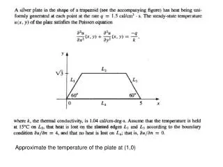
Approximate the temperature of the plate at (1,0). function pdemodel99 [pde_fig,ax]=pdeinit; pdetool('appl_cb',1); pdetool('snapon','on'); set(ax,'DataAspectRatio',[1 1.0499999999999998 1]); set(ax,'PlotBoxAspectRatio',[1.4285714285714286 0.95238095238095255 1.4285714285714286]);

E N D
function pdemodel99 [pde_fig,ax]=pdeinit; pdetool('appl_cb',1); pdetool('snapon','on'); set(ax,'DataAspectRatio',[1 1.0499999999999998 1]); set(ax,'PlotBoxAspectRatio',[1.4285714285714286 0.95238095238095255 1.4285714285714286]); set(ax,'XLim',[-1 1]); set(ax,'YLim',[-1 1]); set(ax,'XTick',[ -1,... -0.90000000000000002,... -0.80000000000000004,... -0.69999999999999996,... -0.59999999999999998,... -0.5,... -0.39999999999999991,... -0.29999999999999993,... -0.19999999999999996,... -0.099999999999999978,... 0,... 0.099999999999999978,... 0.19999999999999996,... 0.29999999999999993,... 0.39999999999999991,... 0.5,... 0.59999999999999998,... 0.69999999999999996,... 0.80000000000000004,... 0.90000000000000002,... 1,... ]); set(ax,'YTick',[ -1,... -0.90000000000000002,... -0.80000000000000004,... -0.69999999999999996,... -0.59999999999999998,... -0.5,... -0.39999999999999991,... -0.29999999999999993,... -0.19999999999999996,... -0.099999999999999978,... 0,... 0.099999999999999978,... 0.19999999999999996,... 0.29999999999999993,... 0.39999999999999991,... 0.5,... 0.59999999999999998,... 0.69999999999999996,... 0.80000000000000004,... 0.90000000000000002,... 1,... ]); pdetool('gridon','on');
pdecirc(0,0,0.3,'C1'); pderect([0 1 0 1],'SQ1'); pdepoly([ 0,0.5,0.5,0.2,0],[ 0,0,0.6,0.3,0.6],'P1');
function pdemodel [pde_fig,ax]=pdeinit; pdetool('appl_cb',1); pdetool('snapon','on'); set(ax,'DataAspectRatio',[1 0.80000000000000004 1]); set(ax,'PlotBoxAspectRatio',[3.75 2.5 1]); set(ax,'XLim',[-1.5 6]); set(ax,'YLim',[-1 3]); set(ax,'XTickMode','auto'); set(ax,'YTickMode','auto'); pdetool('gridon','on'); % Geometry description: pdepoly([ 0,... 5, 4,1,],... [ 0,0, 1.7320508075688772, 1.7320508075688772,... ],... 'P1'); % Mesh generation: setappdata(pde_fig,'trisize',1); setappdata(pde_fig,'Hgrad',1.3); setappdata(pde_fig,'refinemethod','regular'); setappdata(pde_fig,'jiggle',char('on','mean','')); pdetool('initmesh') pdetool('refine') pdetool('refine') pdetool('refine') pdetool('refine') % PDE coefficients: pdeseteq(1,... '1.0',... '0.0',... '1.5/1.04',... '1.0',... '0:10',... '0.0',... '0.0',... '[0 100]') setappdata(pde_fig,'currparam',... ['1.0 ';... '0.0 ';... '1.5/1.04';... '1.0 ']) % Solve parameters: setappdata(pde_fig,'solveparam',... str2mat('0','8064','10','pdeadworst',... '0.5','longest','0','1E-4','','fixed','Inf')) % Plotflags and user data strings: setappdata(pde_fig,'plotflags',[1 1 1 1 1 1 1 1 0 0 0 1 1 0 0 0 0 1]); setappdata(pde_fig,'colstring',''); setappdata(pde_fig,'arrowstring',''); setappdata(pde_fig,'deformstring',''); setappdata(pde_fig,'heightstring',''); % Solve PDE: pdetool('solve') set(findobj(get(pde_fig,'Children'),'Tag','PDEEval'),'String','P1') % Boundary conditions: pdetool('changemode',0) pdesetbd(4,... 'neu',... 1,... '0',... '4') pdesetbd(3,... 'dir',... 1,... '1',... '15') pdesetbd(2,... 'neu',... 1,... '0',... '4') pdesetbd(1,... 'neu',... 1,... '0',... '0')
[pde_fig,ax]=pdeinit; pdecirc(-0.6,0,0.1,'C1'); % center then radius pderect([-0.9 0.9 -0.5 0.5],'R1'); % x-values then y-values set(findobj(get(pde_fig,'Children'),'Tag','PDEEval'),'String','R1-C1')
function pdemodel [pde_fig,ax]=pdeinit; set(ax,'XLim',[-1.5 1.5]); set(ax,'YLim',[-1 1]); set(ax,'XTickMode','auto'); set(ax,'YTickMode','auto'); % Geometry description: pderect([-0.8 0.9 0.6 -0.8],'R1'); pdecirc(-0.7,0.5,0.1,'C1'); pderect([-0.8 -0.7 0.6 0.5],'SQ1'); set(findobj(get(pde_fig,'Children'),'Tag','PDEEval'),'String','R1-SQ1+C1')
Potential Flow Over a Wing When designing aircrafts it is very important to know the areodynamical properties of the wings function g=Airfoil() g=[2 17.7218 16.0116 1.5737 1.6675 1 0 2 16.0116 9.0610 1.6675 1.3668 1 0 2 9.0610 -0.5759 1.3668 -0.1102 1 0 2 -0.5759 -9.5198 -0.1102 -1.8942 1 0 2 -9.5198 -15.6511 -1.8942 -2.5938 1 0 2 -15.6511 -18.1571 -2.5938 -1.7234 1 0 2 -18.1571 -16.9459 -1.7234 0.2051 1 0 2 -16.9459 -12.4137 0.2051 2.2238 1 0 2 -12.4137 -5.4090 2.2238 3.4543 1 0 2 -5.4090 2.8155 3.4543 3.5046 1 0 2 2.8155 10.6777 3.5046 2.6664 1 0 2 10.6777 16.3037 2.6664 1.7834 1 0 2 16.3037 17.7218 1.7834 1.5737 1 0 2 -30.0000 30.0000 -15.0000 -15.0000 1 0 2 30.0000 30.0000 -15.0000 15.0000 1 0 2 30.0000 -30.0000 15.0000 15.0000 1 0 2 -30.0000 -30.0000 15.0000 -15.0000 1 0]' wing = Airfoil(); [p,e,t]=initmesh(wing,'hmax',2); pdemesh(p,e,t)
function r = rvect(p,e,gN) L1=[31,13,30]; %normal u =4 L2=[4,29,12,28,11,27,10,26,2]; % u=15 L3=[25,9,24]; %normal u =4 L4=[1,19,5,20,6,21,7,22,8,23,2]; %normal u =0 np = size(p,2); ne = size(e,2); r = zeros(np,1); for E = 1:ne loc2glb = e(1:2,E); x = p(1,loc2glb); y = p(2,loc2glb); len = sqrt((x(1)-x(2))ˆ2+(y(1)-y(2))ˆ2); xc = mean(x); yc = mean(y); tmp = gN(xc,yc); rK = tmp*[1; 1]*len/2; r(loc2glb) = r(loc2glb) + rK; end