G 1 and G 2 are transfer functions and independent of the inputs, Q ′ and T i ′ .

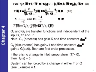
1. G1 and G2 are transfer functions and independent of the inputs, Q′ and Ti′. Note G1 (process) has gain K and time constant t. G2 (disturbance) has gain=1 and time constant t. gain = G(s=0). Both are first order processes. If there is no change in inlet temperature (Ti′= 0), then Ti′(s) = 0. System can be forced by a change in either Ti or Q (see Example 4.1).

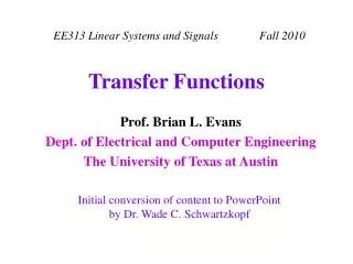
2. Transfer Function Between and Suppose is constant at the steady-state value. Then, Then we can substitute into (10) and rearrange to get the desired TF:

3. Transfer Function Between and Suppose that Q is constant at its steady-state value: Thus, rearranging

4. Comments: • The TFs in (12) and (13) show the individual effects of Q and on T. What about simultaneous changes in both Q and ? • Answer: See (10). The same TFs are valid for simultaneous changes. • Note that (10) shows that the effects of changes in both Q and are additive. This always occurs for linear, dynamic models (like TFs) because the Principle of Superposition is valid. • The TF model enables us to determine the output response to any change in an input. • Use deviation variables to eliminate initial conditions for TF models.

5. Example: Stirred Tank Heater No change in Ti′ Q(0)= 1000cal/sec. Then, step change in Q(t):1500 cal/sec Chapter 4 What is T′(t)?

6. Solve Example 4.1andSolve Example 4.2if you have any questionask me !

7. Properties of Transfer Function Models • Steady-State Gain • The steady-state of a TF can be used to calculate the steady-state change in an output due to a steady-state change in the input. For example, suppose we know two steady states for an input, u, and an output, y. Then we can calculate the steady-state gain, K, from: For a linear system, K is a constant. But for a nonlinear system, K will depend on the operating condition

8. Calculation of K from the TF Model: If a TF model has a steady-state gain, then: • This important result is a consequence of the Final Value Theorem • Note: Some TF models do not have a steady-state gain (e.g., integrating process in Ch. 5)

9. Order of a TF Model • Consider a general n-th order, linear ODE: Take L, assuming the initial conditions are all zero. Rearranging gives the TF:

10. Definition: The order of the TF is defined to be the order of the denominator polynomial. Note: The order of the TF is equal to the order of the ODE. Physical Realizability: For any physical system, in (4-38). Otherwise, the system response to a step input will be an impulse. This can’t happen. Example: n=1 > m=0 Impulse response to step change. Physically impossible.

11. 2nd order process General 2nd order ODE: Laplace Transform: Chapter 4 2 roots : real roots : imaginary roots

12. Examples 1. (no oscillation) Chapter 4 2. (oscillation)

13. G1(s) Y(s) G2(s) • Additive Property • Suppose that an output is influenced by two inputs and that the transfer functions are known: Then the response to changes in both and can be written as: The graphical representation (or block diagram) is: U1(s) U2(s)

14. Multiplicative Property • Suppose that, Then, Substitute, Or,

15. Example 1: Place sensor for temperature downstream from heated tank (transport lag) Distance L for plug flow, Dead time Chapter 4 V = fluid velocity Tank: Sensor: is very small (neglect) Overall transfer function:

16. Solve Example 4.3andSolve Example 4.4if you have any questionask me !

17. Chapter 4

18. Chapter 4