Download
1 / 170
1.72k likes | 2.34k Views
BIO-201. ECOLOGY Communities and Ecosystems. H.J.B. Birks. Communities and Ecosystems. Species Abundance, Diversity, & Community Ecology Community Ecology and Dynamics Ecosystem Ecology – Energy Flux Ecosystem Ecology – Matter Flux Long-term Ecology (=Ecological Palaeoecology)

E N D
BIO-201 ECOLOGYCommunities and Ecosystems H.J.B. Birks
Communities and Ecosystems • Species Abundance, Diversity, & Community Ecology • Community Ecology and Dynamics • Ecosystem Ecology – Energy Flux • Ecosystem Ecology – Matter Flux • Long-term Ecology (=Ecological Palaeoecology) • Broad-scale Ecology – World Vegetation Biomes • Broad-scale Ecology – Landscape & Geographical Ecology • Broad-scale Ecology – Species Richness Patterns in Time • Broad-scale Ecology – Species Richness Patterns in Space • Broad-scale Ecology – Global Earth-System Ecology
BIO-201 ECOLOGY 1. Species Abundance, Diversity, and Community Ecology H.J.B. Birks
Species Abundance, Diversity, and Community Ecology Sub-divisions of ecology Scales in ecology Community level of ecological organisation Important concepts about community level of organisation The study of communities How do we quantify the number & relative abundance of species in communities? - Species abundances - Rank-abundance curves - Species numbers (= richness) and species diversity - Not all species are equal! What determines diversity? - Environmental complexity - Disturbance and diversity What determines community structure? Different concepts of the community How to analyse community-scale data? Conclusions and summary
Pensum The lecture, of course, and the PowerPoint handouts of this lecture on the BIO-201 Student Portal Also ‘Topics to Think About’ on the Student Portal filed under projects
Topics to Think About On the Bio-201 Student Portal filed under Projects, there are several topics to think about for each lecture. These topics are designed to help you check that you have understood the lecture and to identify important topics for discussion in the Bio-201 colloquia. In addition, there are two or three more demanding questions at the sort of level you can expect in the examination question based on my 10 lectures. These can also be discussed in the colloquia.
Background Information There is now a wealth of good or very good ecology textbooks but perhaps no excellent, complete, or perfect textbook of ecology. Not surprising, given just how diverse a subject ecology is in space and time and all their scales. This lecture draws on primary research sources, my own knowledge, experience, observations, and studies, and several textbooks.
Textbooks that provide useful background material for this lecture Begon, M. et al. (2006) Ecology. Blackwell (Chapter 16, parts of Chapters 19 & 20) Bush, M. (2003) Ecology of a Changing Planet. Prentice Hall (Chapter 15) Krebs, C.J. (2001) Ecology. Benjamin Cummings (Chapters 20, 22, 23) Miller, G.T. (2004) Living in the Environment. Thomson (Chapter 8) Molles, M.C. (2007) Ecology Concepts and Applications. McGraw-Hill (Chapter 16) Ricklefs, R.E. & Miller, G.L. (2000) Ecology. W.H. Freeman (Chapters 26, 27, 29) Smith, R.L. & Smith, T.M. (2007) Ecology and Field Biology. Benjamin Cummings (Chapter 20) Townsend, C.R. et al. (2008) Essentials of Ecology. Blackwell (Chapters 9, 10)
A Reminder If you try to read Begon, Townsend, and Harper (2006) Ecology – From Individuals to Ecosystems, there is a 17-page glossary of the very large (too large!) number of technical words used in the book on the Bio-201 Student Portal. It can be downloaded from the File Storage folder. Good luck!
Sub-Divisions of Ecology • Functional ecology and evolutionary ecology • Modern ecology and long-term ecology (=palaeoecology) (the Fourth dimension of ecology) • Autecology – study of ecological relationships of a single species • Synecology – study of all the species living together as a community (group of plants and animals in a given place forming ecological units of various sizes and degrees of interrelation and integration) • Pure and applied ecology • "Pure"– understand, for understanding's sake, the processes responsible for determining the structure and composition of particular assemblages or communities • "Applied"– ecology relevant to food gathering and production, conservation, control of pests and pathogens, pollution, preservation of biodiversity, etc. Includes conservation ecology and restoration ecology.
Descriptive ecology – basic patterns of what grows where, what are the environmental variables, and what is the inherent variation in space and time • Explanatory ecology - underlying processes behind observed patterns. Processes may be proximal (near) or ultimate (final) • Predictive ecology – use ecological knowledge and understanding to predict how organisms will respond to environmental changes • Observational or field ecology – 'scientific natural history' • Laboratory experimental ecology – 'simplified ecology' • Field experimental ecology – most difficult to do • Behavioural ecology – individuals • Population ecology – populations • Community ecology – communities • Landscape ecology – landscapes • Geographical ecology – mappable features • Global ecology – biomes and Earth's systems
Ecology is like a giant and complex jigsaw puzzle If the organism is not a predator, 'prey' is replaced by 'food' or if the organism is a plant, 'prey' is replaced by 'light and nutrients'. In addition, an organism competes with other organisms (competitors) for food. In reality a multi-dimensional (and unsolvable!) jigsaw-puzzle and we do not have all the pieces!
Biosphere Biosphere landscapes Communities Populations Individual Scales in Ecology Biological or hierarchical scales Biosphere Biomes e.g. rainforest Ecosystems & Landscapes Communities Species Populations; breeding individuals Individual organisms
Atmosphere Biosphere Vegetation and animals Soil Crust Rock core Lithosphere Mantle Crust (soil and rock) Crust Biosphere (Living and dead organisms) Atmosphere (air) Hydrosphere (water) Lithosphere (crust, top of upper mantle) Global Scale (Lectures 6, 10) Biosphere Hydrosphere (Lithosphere)
Coastal chaparral and scrub Coniferous forest Desert Coniferous forest Prairie grassland Deciduous forest Appalachian Mountains Mississippi River Valley Great Plains Rocky Mountains Great American Desert Sierra Nevada Mountain Coastal mountain ranges 15,000 ft 10,000 ft Average annual precipitation 5,000 ft 100-125 cm (40-50 in.) 75-100 cm (30-40 in.) 50-75 cm (20-30 in.) 25-50 cm (10-20 in.) below 25 cm (0-10 in.) Broad Spatial or Biome Scale (Lecture 6) World Vegetation Types or Biomes Role of climate
Landscape Scale (Lecture 7) Coast-mountain transition in western Norway
Geographical Scale (Lecture 7) Elevation gradient = gradual change Alpine tundra Montane coniferous forest Deciduous forest SEA Temperate forest
Community Scale (Lectures 1, 2) Populations of different species living and interacting within an ecosystem are referred to collectively as a community Often no real boundaries between communities
Land zone Transition zone Aquatic zone Number of species Species in land zone Species in aquatic zone Species in transition zone only Community Boundaries: Often Gradual
Deciduous forest and rocky shore = sharp change between communities
Scales of relevance in these ten lectures on Communities and Ecosystems Community scale (Lectures 1, 2) Ecosystem (Lectures 3, 4), Landscape (Lecture 7), and Geographical (Lectures 7, 8, 9) scales Biome scale (Lecture 6) Biosphere or Global scale (Lecture 10) plus Time dimension (long-term ecology or palaeoecology) (Lectures 5, 8)
Spatial and Temporal Scales of Biodiversity –closely related
Biosphere Biosphere Ecosystems Communities Populations Organisms Today’s Ecological Scale Biosphere Biomes Ecosystems & Landscapes COMMUNITIES Species Populations Organisms
Community Level of Ecological Organisation 'Group of plants and animals in a given place and time forming ecological units of various sizes and degrees of inter-relation and integration.' Community concept first applied to plants, more recently applied to animals. Most definitions only refer to plants. 'an aggregate of living plants having mutual relations among themselves and to the environment' (Oosting, 1956) 'a collection of plant populations found in one habitat type in one area, and integrated to a degree by competition, complementarity, and dependence' (Grubb, 1987)
Important Concepts about Community Level of Organisation • Collections of species which occur together in some common environment or habitat type. • Organisms making up the community are somehow integrated and may interact as a unit. • Communities are not constructed only of plants. • Some communities are mostly animals (e.g. fish and invertebrates that comprise coral-reef communities). • Most communities consist of a mixture of plants, animals, fungi, prokaryotes, and protoctists. • Population dynamics, distribution and abundance, growth and life histories, competition, predation, herbivory, parasitism, disease, and mutualism provide basic processes within assemblages of living organisms that generate the observed patterns of species diversity, abundance, and composition at the community level.
Recognition of communities – two main ways • (a) environment or habitat where community occurs (e.g. lakes, sand-dunes, coastal rock pools) • (b) largest or most abundant or prominentspecies (e.g. pine forest, oak woodland, grassland, Sphagnum bog) • Size of community – no fixed size, can range from very small and constrained (e.g. association of micro-organisms in mammalian gut) to huge expanses of grassland and forest. • Why are similar groups of species found again and again in similar habitats? • If the habitat provides a collection of environmental niches and if the same niches occur in similar habitats, then they will be filled by the same species. • Niches for particular plants, grazing animals, decomposers, parasites, etc.
Community is built up of species with other dependent species in recognisable combinations. • But communities found in a particular habitat type will not be identical. Minordifferences in the environment that vary continuously in space and time may occur. Effects of chance or history of the site may mean that some species usually found together are missing and other more unusual species may be present. • Species present in a community will vary depending on where in the world the particular community is found. Species growing in coastal pools on rocky shores in Australia will be different from species growing in similar pools in Norway. Hence the importance of biogeography and geographical ecology in determining the available species pool. • However, wherever rock pools occur, expect them to have similar relationships between species occupying the same collection of niches.
14. Species that assemble to form a community are determined by (i) dispersal constraints, (ii) environmental constraints, and (iii) internal dynamics. Species pools: Total Pool – function of evolution and history Habitat Pool – function of environmental constraints Geographic Pool – function of dispersal constraints Ecological Pool – function of internal dynamics Community – what remains in face of biotic interactions
The Study of Communities Within any community there is a complex series of interactions between individuals of different species. The whole collection of populations may fit together into a functional unit; the community. Community ecology seeks to understand the way species groupings are distributed in nature and the ways that these groupings are influenced by their abiotic environment (Part I of this course) and by interactions between species populations (Part II) How do we study communities and understand the complexity of such systems?
What is the community structure? • - abiotic features noted (e.g. marine, freshwater, marsh, desert; geology; topography; climate, etc.) • - overall form described (e.g. terrestrial life forms such as trees, shrubs, herbs and grasses, mosses; aquatic mode of locomotion such as free swimmers, planktonic drifters, bottom dwellers, sessile adults) • What species are present? • How many species live in the community? (Diversity) Is it species-poor or species-rich? • What are the abundance patterns of the species?
How does the community function? Trophic food webs within the community can be investigated to assess the importance of primary producers, herbivores, predators, and decomposers. This provides data on energy and nutrient cycles. See lectures on Ecosystem Ecology (Lectures 3, 4). • What is the influence of the abiotic environment on the composition and structure? • How does the community regenerate and sustain itself? Population dynamics and stability (Lecture 2). • What is the history of the community? Long-term ecology or palaeoecology (Lecture 5).
No community is well enough studied that we can answer these eight questions! Overall community structure will be determined by features of the physical environment, community size, longevity of the species present, and history. Community may be stable or unstable, have low or high primary productivity, and may change seasonally or even daily. Community, ecosystem, and broad-scale ecology are very difficult to study.
How do we study community ecology? • Search for patterns in the collective and emergent properties • Collective properties – species richness and diversity, community biomass • Emergent properties – stability, resilience, dynamics • (e.g. for cake • - numbers or size of ingredients = collective properties; • - taste and texture = emergent properties)
Patterns are repeated consistencies, such as repeated groupings of similar growth-forms or species in different places, or repeated trends in richness along different environmental gradients. • Recognition of patterns leads to formulation of hypotheses about the causes of the patterns, so-called processes. • Test hypotheses by making further independent observations or by doing experiments. • Much of community ecology is, by necessity, descriptive or narrative, rather than analytical with strict hypothesis testing or statistical modelling.
Communities can be defined & studied and the underlying processes identified at many scales • Global scale – boreal forest biome • Strong climate control • Boreal forest in Norway is represented by communities dominated by Pinus (furu), Picea (gran), and Pinus and Picea • Strong soil, topographical, and historical controls • At a finer scale, the field layer may differ between different Pinus stands • Strong soil or historical (e.g. fire) controls • At an even finer scale, within a Pinus stand there are animals that inhabit fallen and rotting logs, plants and animals that live in the gut of the deer in the forest, etc. • The scale of investigation depends on the ecological questions being asked.
The structure of oak (Quercus) woodland in spring and summer Chapman & Reiss
A cross-section of a typical rock pool showing the mixed nature of the community and some of the other organisms which inhabit the more open rocky shore. Chapman & Reiss
The general structure of the mammalian gut and common members of gut communities (not to scale). Chapman & Reiss
Often difficult to study large numbers of species, so community ecologists may work with restricted groups, e.g. plants, insects. Some focus on guilds – group of organisms that all make their living in a similar way (e.g. seed-eating animals in a desert, fruit-eating birds in a forest, filter-feeding invertebrates in a stream). Some guilds consist of closely related species; others may be taxonomically unrelated. For example, fruit-eating birds on South Pacific Islands are mainly pigeons, whilst the same guild in USA deserts consists of mammals, birds, and ants. Guild concept mainly used by animal ecologists. Life-form or growth-form or functional type used by plant ecologists. Combination of structure and growth-dynamics (e.g. trees, vines, annual plants, grasses, herbs (= forbs)). Like an animal guild, plants of similar life-form exploit the environment in similar ways. By studying animal guilds or plant life-forms, communities can be studied in a more manageable and coherent way than trying to consider all species simultaneously.
All communities have attributes or features that differ from those of the components that make up the community and that only have meaning with reference to the collective assemblage or community. These attributes are • Number of species • Relative abundance of species • Nature of their interactions • Physical structure, defined primarily by the growth-forms of the plant components of the community
How do we Quantify the Number & Relative Abundance of Species in Communities? Species Abundances One of the most striking features of communities is the variation in the relative abundance of species. Basic questions often asked: • For a given community, how many species are there and what are their relative abundances? • How many species are rare? • How many species are common?
Species abundances are usually based on individuals per species, or variables such as percentage cover or biomass. Fundamental aspect of community structure – "minimal community structure" (Sugihara, 1980) What will be found if we go to a community and quantify the abundance of species within a group of taxonomically or ecologically related organisms such as birds, shrubs, herbs, or diatoms?
Species abundance data are arranged in the form of a species abundance distribution, that is a frequency distribution of the number of species with X = 1, 2, 3, … r individuals. Insect count data from grassland based on 14 sweep nets X= number of individuals per species f= frequency of species in each of the X classes There are 389 individuals and 69 species.
Can we fit a statistical distribution model to such species abundance data? • Hope to find a 'general' model requiring a few, easily estimated and ecologically meaningful parameters. • Turns out that there are regularities in the relative abundance of species in many different communities. If you can thoroughly sample the community, there are usually: • a few very abundant species • a few very rare species • most species have a moderate abundance
Preston "distribution of commonness and rarity" and the log-normal distribution (1948, 1962) Consider abundance in relative terms and say that one species is twice as abundant as another. Graph the abundance of species in samples as frequency distribution where the species abundance intervals are 0-1, 1-2, 2-4, 4-8, 8-16, 16-32, etc. individuals, so-called octaves. Frank Preston
Insect data – 389 individuals, 69 species OctaveS(R) number of species in Rth octave (oct) Octave 1 (0-1) 32/2 = 16 Octave 2 (1-2) 16 (from oct 1) + (8/2) = 20 Octave 3 (2-4) 4 (from oct 2) + 9 + (2/2) = 14 Octave 4 (4-8) 1 (from oct 3) + 3 + 3 + 3 + 0 = 10 Octave 5 (8-16) 2 + 1 + 2 = 5 Note that abundance classes falling on the lines separating consecutive octaves (1, 2, 3) are split between octaves
In Preston log-normal distribution, plot the abundance classes on log2 scale (log2 of 1 = 0, log2 of 2 = 1, log2 of 4 = 2, log2 of 8 = 3, etc.). Each class represents a doubling of the previous abundance class. Plot log2 of species abundance against the number of species in each abundance interval. Each abundance interval is twice the preceding one.
Log-normal distribution is whereS(R)is the number of species in the Rth octave from the mode S0is an estimate of the number of species in the modal octave (the octave with the most species) ais an inverse measure of the width of the distribution (a = ½whereis the standard deviation) eis exponential function or antilog
Estimation of parameters S0 and a where S(o) is the observed number of species in the modal octave and S(Rmax) is the observed number of species in the octave most distant from the modal (indicated by Rmax) Parameter a has been found to be about 0.2 for a large number of samples in ecology. It has been shown that this ‘rule’ may be a product of the mathematical properties of the log-normal distribution. As the total number of species in the community varies from 20 to 10000, a will vary from 0.3 to 0.13 (assuming that the underlying distribution follows the so-called ‘canonical log-normal’ distribution).
An estimate of S0 is obtained either by fixing it at the observed value for the number of species in the modal octave, S(o), or by estimating it where lognS (R) is the mean of the logarithm of the observed number of species per octave, a is estimated as above, and R2 is the mean of all the R2s.