Download
1 / 35
350 likes | 486 Views
Linear Sorting. Sorting in O( n ). Previously. Previous sorts had the same property: they are based only on comparisons Any comparison-based sorting algorithm must run in Ω( n log n ) Thus, M ERGE S ORT and H EAP S ORT are asymptotically optimal

E N D
Linear Sorting Sorting in O(n) Jeff Chastine
Previously • Previous sorts had the same property: they are based only on comparisons • Any comparison-based sorting algorithm must run in Ω(n log n) • Thus, MERGESORT and HEAPSORT are asymptotically optimal • Obviously, this lower bound does not apply to linear sorting Jeff Chastine
Lower Bound for Sorting • Assume (for simplicity) that all elements in an input sequence a1, a2, ..., an are distinct • We can view comparison-based sorting using a decision tree • Any correct sorting algorithm must be able to handle any of the n! permutations • Each permutation must appear as a leaf in the tree Jeff Chastine
The Decision Tree a1:a2 > ≤ a2:a3 a1:a3 ≤ > ≤ > a2:a3 a1:a3 1,2,3 2,1,3 ≤ ≤ > > 2,3,1 1,3,2 3,1,2 3,2,1 a1 = 6, a2 = 8, a3 = 5 Jeff Chastine
Proof • Consider a decision tree with height h with l reachable leaves • n! l • Since a binary tree of height h has no more than 2h leaves: • n! l 2h • Taking the log of both sides: • h lg (n!) = (n lg n) Jeff Chastine
Counting Sort • Each element is an integer in the range from 1 to k • For each element, determine the number of elements less than it • Works well on small ranges • Does not sort in place Jeff Chastine
1 2 3 4 5 6 7 8 A Original 3 6 4 1 3 4 1 4 1 2 3 4 5 6 Number of 1's, 2's.. C 2 0 2 3 0 1 How do you construct C's size? How do you fill C's data? Jeff Chastine
Modify CSuch that C now tells how many elements are less than i 1 2 3 4 5 6 Number of 1's, 2's.. C 2 0 2 3 0 1 1 2 3 4 5 6 Number of slots C' 2 2 4 7 7 8 How do you construct C'? Jeff Chastine
Move into B from A 1 2 3 4 5 6 7 8 A Original 3 6 4 1 3 4 1 4 1 2 3 4 5 6 7 8 B Sorted 1 2 3 4 5 6 Number of slots. C 2 2 4 7 7 8 Jeff Chastine
Move into B from A 1 2 3 4 5 6 7 8 A Original 3 6 4 1 3 4 1 4 1 2 3 4 5 6 7 8 B Sorted 4 1 2 3 4 5 6 Number of slots. C 2 2 4 6 7 8 Jeff Chastine
Move into B from A 1 2 3 4 5 6 7 8 A Original 3 6 4 1 3 4 1 4 1 2 3 4 5 6 7 8 B Sorted 4 1 2 3 4 5 6 Number of slots. 2 C 2 4 6 7 8 Jeff Chastine
Move into B from A 1 2 3 4 5 6 7 8 A Original 3 6 4 1 3 4 1 4 1 2 3 4 5 6 7 8 B Sorted 1 4 1 2 3 4 5 6 Number of slots. 1 C 2 4 6 7 8 Jeff Chastine
Move into B from A 1 2 3 4 5 6 7 8 A Original 3 6 4 1 3 4 1 4 1 2 3 4 5 6 7 8 B Sorted 1 4 1 2 3 4 5 6 Number of slots. C 1 2 4 6 7 8 Jeff Chastine
Move into B from A 1 2 3 4 5 6 7 8 A Original 3 6 4 1 3 4 1 4 1 2 3 4 5 6 7 8 B Sorted 1 4 4 1 2 3 4 5 6 Number of slots. C 1 2 4 5 7 8 Jeff Chastine
Move into B from A 1 2 3 4 5 6 7 8 A Original 3 6 4 1 3 4 1 4 1 2 3 4 5 6 7 8 B Sorted 1 4 4 1 2 3 4 5 6 Number of slots. C 1 2 4 5 7 8 Jeff Chastine
Move into B from A 1 2 3 4 5 6 7 8 A Original 3 6 4 1 3 4 1 4 1 2 3 4 5 6 7 8 B Sorted 1 3 4 4 1 2 3 4 5 6 Number of slots. C 1 2 3 5 7 8 Jeff Chastine
Move into B from A 1 2 3 4 5 6 7 8 A Original 3 6 4 1 3 4 1 4 1 2 3 4 5 6 7 8 B Sorted 1 3 4 4 1 2 3 4 5 6 Number of slots. C 1 2 3 5 7 8 Jeff Chastine
Move into B from A 1 2 3 4 5 6 7 8 A Original 3 6 4 1 3 4 1 4 1 2 3 4 5 6 7 8 B Sorted 1 1 3 4 4 1 2 3 4 5 6 Number of slots. C 0 2 3 5 7 8 Jeff Chastine
Move into B from A 1 2 3 4 5 6 7 8 A Original 3 6 4 1 3 4 1 4 1 2 3 4 5 6 7 8 B Sorted 1 1 3 4 4 1 2 3 4 5 6 Number of slots. C 0 2 3 5 7 8 Jeff Chastine
Move into B from A 1 2 3 4 5 6 7 8 A Original 3 6 4 1 3 4 1 4 1 2 3 4 5 6 7 8 B Sorted 1 1 3 4 4 4 1 2 3 4 5 6 Number of slots. C 0 2 3 4 7 8 Jeff Chastine
Move into B from A 1 2 3 4 5 6 7 8 A Original 3 6 4 1 3 4 1 4 1 2 3 4 5 6 7 8 B Sorted 1 1 3 4 4 4 1 2 3 4 5 6 Number of slots. C 0 2 3 4 7 8 Jeff Chastine
Move into B from A 1 2 3 4 5 6 7 8 A Original 3 6 4 1 3 4 1 4 1 2 3 4 5 6 7 8 B Sorted 1 1 3 4 4 4 6 1 2 3 4 5 6 Number of slots. C 0 2 3 4 7 7 Jeff Chastine
Move into B from A 1 2 3 4 5 6 7 8 A Original 3 6 4 1 3 4 1 4 1 2 3 4 5 6 7 8 B Sorted 1 1 3 4 4 4 6 1 2 3 4 5 6 Number of slots. C 0 2 3 4 7 7 Jeff Chastine
Move into B from A 1 2 3 4 5 6 7 8 A Original 3 6 4 1 3 4 1 4 1 2 3 4 5 6 7 8 B Sorted 1 1 3 3 4 4 4 6 1 2 3 4 5 6 Number of slots. C 0 2 2 4 7 7 Jeff Chastine
The Code COUNTING-SORT (A, B, k) fori←1 tok // Init C doC[i] ←0 // (k) forj←1 tolength[A] // Build C doC[A[j]] ←C[A[j]] + 1 // (n) fori ← 2 tok // Make C' doC[i] ←C[i] + C[i-1] // (k) forj←length[A] downto 1 // Copy info doB[C[A[j]]] ←A[j] // (n) C[A[j]] ←C[A[j]] -1 Jeff Chastine
Stable Sorting • An important property (for later) is that counting sort is stable: • numbers with the same value appear in the output array in same order they did in the input array • This is important for our next sorting algorithm: radix sort Jeff Chastine
Radix Sort • Sorting by "column" • A d-digit number would create d columns • Start with least-significant row • Usually requires counting sort to be used on the columns Jeff Chastine
Example(by hand) H H H 331 429 190 127 982 784 318 190 331 982 784 127 318 429 318 127 429 331 982 784 190 127 190 318 331 429 784 982 F F F Jeff Chastine
The Code RADIX-SORT (A, d) fori← 1 tod do use a stable sort to sort A on digit i • Have we created d more times work than counting sort? • If so, why do we do this? Jeff Chastine
Analysis • Each digit is in the range 0 – (k-1) • Takesktime to constructC • Each pass over nd-digit numbers takes (n+k) • Thus, the total running time is (d(n+k)) Jeff Chastine
Bucket Sort • Once again, not any greater than counting sort • Assumes uniform distribution of random numbers [0, 1) • "Chunk" numbers into equal-sized buckets, based on first digit • Sort the buckets (with what?) Jeff Chastine
Example → .06 0 / 1 .06 / 2 → .43 .37 3 → → → .48 .43 .44 .48 4 .37 / 5 .91 / 6 .44 / 7 / .98 8 → .98 9 Jeff Chastine
The Code BUCKET-SORT (A) n←length[A] for i← 1 to n do insert A[i] into list B[A[i]] for i ← 0 to n - 1 do sort list B[i] with insertion sort concatenate the lists together Jeff Chastine
Proof of Bucket Sort • Consider two elements A[i] and A[j] • Assume A[i] A[j] • Then, A[i] is placed into either the same bucket, or a bucket with a lower index. • The sort of each bucket guarantees A[i] and A[j] are ordered correctly Jeff Chastine
Of Interest(only to me) • “As long as the input has the property that the sum of the squares of the bucket sizes is linear in the total number of elements”... “bucket sort will run in linear time” • In other words, each bucket should get the square root of the number of bucket elements. Jeff Chastine