Linear Time Sorting: Counting Sort and Radix Sort Explained
This document discusses linear time sorting algorithms, focusing on Counting Sort and Radix Sort. While comparison-based sorts like Merge Sort and Quicksort have a worst-case time complexity of O(n log n), Counting Sort operates without comparisons, achieving O(n+k) time complexity under specific conditions. Radix Sort further allows digit-based sorting, enhancing efficiency for data with fixed-size keys. A detailed analysis of the algorithms is provided, along with pseudo-code, demonstrating their uniqueness and practical applications in sorting tasks.

Linear Time Sorting: Counting Sort and Radix Sort Explained
E N D
Presentation Transcript
Q:Is O(n lg n) the best we can do? A: Yes, as long as we use comparison sorts How fast can we sort? All the sorting algorithms we have seen so far are comparison sorts: only use comparisons to determine the relative order of elements. • E.g., insertion sort, merge sort, quicksort, heapsort. The best worst-case running time that we’ve seen for comparison sorting is O(nlgn).
Sorting in linear time Counting sort: No comparisons between elements. • Input: A[1 . . n], where A[j]{1, 2, …, k}. • Output: B[1 . . n], sorted. • Auxiliary storage: C[1 . . k].
Counting sort fori 1tok doC[i] 0 forj 1ton doC[A[j]] C[A[j]] + 1⊳C[i] = |{key = i}| fori 2tok doC[i] C[i] + C[i–1]⊳C[i] = |{key i}| forjndownto1 doB[C[A[j]]] A[j] C[A[j]] C[A[j]] – 1
4 1 3 4 3 Counting-sort example 1 2 3 4 5 1 2 3 4 A: C: B:
4 1 3 4 3 0 0 0 0 Loop 1 1 2 3 4 5 1 2 3 4 A: C: B: fori 1tok doC[i] 0
4 1 3 4 3 0 0 0 1 Loop 2 1 2 3 4 5 1 2 3 4 A: C: B: forj 1ton doC[A[j]] C[A[j]] + 1⊳C[i] = |{key = i}|
4 1 3 4 3 1 0 0 1 Loop 2 1 2 3 4 5 1 2 3 4 A: C: B: forj 1ton doC[A[j]] C[A[j]] + 1⊳C[i] = |{key = i}|
4 1 3 4 3 1 0 1 1 Loop 2 1 2 3 4 5 1 2 3 4 A: C: B: forj 1ton doC[A[j]] C[A[j]] + 1⊳C[i] = |{key = i}|
4 1 3 4 3 1 0 1 2 Loop 2 1 2 3 4 5 1 2 3 4 A: C: B: forj 1ton doC[A[j]] C[A[j]] + 1⊳C[i] = |{key = i}|
4 1 3 4 3 1 0 2 2 Loop 2 1 2 3 4 5 1 2 3 4 A: C: B: forj 1ton doC[A[j]] C[A[j]] + 1⊳C[i] = |{key = i}|
4 1 3 4 3 1 0 2 2 1 1 2 2 B: Loop 3 1 2 3 4 5 1 2 3 4 A: C: C': fori 2tok doC[i] C[i] + C[i–1]⊳C[i] = |{key i}|
4 1 3 4 3 1 0 2 2 1 1 3 2 B: Loop 3 1 2 3 4 5 1 2 3 4 A: C: C': fori 2tok doC[i] C[i] + C[i–1]⊳C[i] = |{key i}|
4 1 3 4 3 1 0 2 2 1 1 3 5 B: Loop 3 1 2 3 4 5 1 2 3 4 A: C: C': fori 2tok doC[i] C[i] + C[i–1]⊳C[i] = |{key i}|
4 1 3 4 3 1 1 3 5 3 1 1 2 5 Loop 4 1 2 3 4 5 1 2 3 4 A: C: B: C': forjndownto1 doB[C[A[j]]] A[j] C[A[j]] C[A[j]] – 1
4 1 3 4 3 1 1 2 5 3 4 1 1 2 4 Loop 4 1 2 3 4 5 1 2 3 4 A: C: B: C': forjndownto1 doB[C[A[j]]] A[j] C[A[j]] C[A[j]] – 1
4 1 3 4 3 1 1 2 4 3 3 4 1 1 1 4 Loop 4 1 2 3 4 5 1 2 3 4 A: C: B: C': forjndownto1 doB[C[A[j]]] A[j] C[A[j]] C[A[j]] – 1
4 1 3 4 3 1 1 1 4 1 3 3 4 0 1 1 4 Loop 4 1 2 3 4 5 1 2 3 4 A: C: B: C': forjndownto1 doB[C[A[j]]] A[j] C[A[j]] C[A[j]] – 1
4 1 3 4 3 0 1 1 4 1 3 3 4 4 0 1 1 3 Loop 4 1 2 3 4 5 1 2 3 4 A: C: B: C': forjndownto1 doB[C[A[j]]] A[j] C[A[j]] C[A[j]] – 1
Analysis fori 1tok doC[i] 0 (k) forj 1ton doC[A[j]] C[A[j]] + 1 (n) fori 2tok doC[i] C[i] + C[i–1] (k) forjndownto1 doB[C[A[j]]] A[j] C[A[j]] C[A[j]] – 1 (n) (n + k)
Running time If k = O(n), then counting sort takes (n) time. • But, sorting takes (nlgn) time! • Where’s the fallacy? Answer: • Comparison sorting takes (nlgn) time. • Counting sort is not a comparison sort. • In fact, not a single comparison between elements occurs!
4 1 3 4 3 A: 1 3 3 4 4 B: Stable sorting Counting sort is a stable sort: it preserves the input order among equal elements.
Radix sort • Origin: Herman Hollerith’s card-sorting machine for the 1890 U.S. Census. (See Appendix .) • Digit-by-digit sort. • Hollerith’s original (bad) idea: sort on most-significant digit first. • Good idea: Sort on least-significant digit first with auxiliary stable sort.
3 2 9 7 2 0 7 2 0 3 2 9 4 5 7 3 5 5 3 2 9 3 5 5 6 5 7 4 3 6 4 3 6 4 3 6 8 3 9 4 5 7 8 3 9 4 5 7 4 3 6 6 5 7 3 5 5 6 5 7 7 2 0 3 2 9 4 5 7 7 2 0 3 5 5 8 3 9 6 5 7 8 3 9 Operation of radix sort
7 2 0 3 2 9 3 2 9 3 5 5 4 3 6 4 3 6 8 3 9 4 5 7 • Sort on digit t 3 5 5 6 5 7 4 5 7 7 2 0 6 5 7 8 3 9 Correctness of radix sort Induction on digit position • Assume that the numbers are sorted by their low-order t – 1 digits.
7 2 0 3 2 9 3 2 9 3 5 5 4 3 6 4 3 6 8 3 9 4 5 7 • Two numbers that differ in digit t are correctly sorted. • Sort on digit t 3 5 5 6 5 7 4 5 7 7 2 0 6 5 7 8 3 9 Correctness of radix sort Induction on digit position • Assume that the numbers are sorted by their low-order t – 1 digits.
7 2 0 3 2 9 3 2 9 3 5 5 4 3 6 4 3 6 8 3 9 4 5 7 • Sort on digit t 3 5 5 6 5 7 4 5 7 7 2 0 6 5 7 8 3 9 Correctness of radix sort Induction on digit position • Assume that the numbers are sorted by their low-order t – 1 digits. • Two numbers that differ in digit t are correctly sorted. • Two numbers equal in digit t are put in the same order as the input correct order.
RADIX SORT ALGORITHM • RADIX_SORT(A,d) • For i 1to d • do use stable sort to sort array A on digit i
Bucket Sort • Pseudo code of Bucket sort is: