Download

1 / 34
340 likes | 477 Views
Section 5. Chesapeake Bay Network Generation. CB watershed ~ 64,000 square miles ~ 166,000 square kilometers Constructed 3 models Version I ERF1, ~1300 stream reaches 1K DEM Versions II and III Stream and watershed network created from 30m DEM Used ERF1 stream-characteristics

E N D
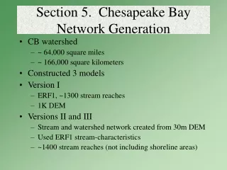
Section 5. Chesapeake Bay Network Generation • CB watershed • ~ 64,000 square miles • ~ 166,000 square kilometers • Constructed 3 models • Version I • ERF1, ~1300 stream reaches • 1K DEM • Versions II and III • Stream and watershed network created from 30m DEM • Used ERF1 stream-characteristics • ~1400 stream reaches (not including shoreline areas)
Stream Reach Characteristics Mean streamflow Mean velocity Travel time Unique reach ID Networked Topological Properties Trace up and down stream Relative Consistent Density Stream Density No Stream Reach Characteristics ERF1 Reach File is Building Block 100K Issues 100K DLG, RF3 & NHD
CHESAPEAKE BAY NETWORK GENERATIONVERSION II, 1992 • Generate New Stream Network • Flow Direction from 30m DEM (NED) • Flow Accumulation > 5000 cells = New Reach • Add/Correct Reaches • Select Out Reaches Corresponding to RF1 • Conflate ERF1 Attributes to New Reach Network • Add Nodes to Reach at Monitoring Station • Divide Shoreline in Arbitrary Locations • Generate Watershed Boundaries for Each Reach • Estimate Travel times for New Reaches and Shoreline
Flow Direction 32 64 128 16 1 8 4 2 8 Direction of flow from cell to cell 4 4 1 4 4 4 4 16 16 16 16 2 8 4
Flow Accumulation 5001 5010 5030 5040 5041 5043 10 0 5050 1 0 6200 6030 6005 6001 6000 950 949 0 6210 6220 6221 Number of cells flowing into a cell 5000 cells constitutes a stream-water pathway (reach) 30m resolution
GRID Condition statement Con (FLOWGRID > 5000, 1) Process entire watershed Convert GRID cells representing pathway into vector (line)
New Stream Reach Generation • Stream Channel now Corresponds with Topography • Produces more than necessary • Used for stream density variable • White – “New Streams” • Blue – Keep for Model Box Area ~ 209 km2
100k NHD, RF1, and New Reach Network • White– 100k • Red– RF1 • Blue - New
Select and keep main water channel relevant to RF1 scale Selecting Main Stream Channel • Corrects location of streams • ½ km offset • Red – RF1 • Blue – New Stream Network
Delaware Add/Correct Reaches • Eastern Shore Nanticoke R. • Ditching • Very Flat • Used 100k for corrections • Wide Rivers and Reservoirs
3 Topology 1 2 4 Trace used to check connectivity of network Finds ‘Arcs” flowing in wrong direction that causes break in network AE “FLIP” command issued Network PropertiesDigitalStream Reaches
Manage attributes by reach and arc Multiple arcs per reachDigitalStream Reaches Length = L1 + L2 + L3 Reach 3121 L3 + + L2 L1 ARC# 3 ARC# 2 ARC# 1 ARC#1 - 3121 ARC#2 - 3121 ARC#3 - 3121 4 3 2 1
Conflation of Attributes Reach-ID = 3121 • AML/Menu interface in ArcEdit • Select RF1 (ERF1) reach to obtain unique number • Select new reach & establish one-to-one relationship CALC Reach-ID = 3121 • Relate file & transfer attributes
Network ConstructionSpatially Referencing Monitoring Stations • Adding Nodes at Station Locations (Split.aml) • Attributing Reaches with STAID (Split.aml) • Attributing Unique Reach ID (ERF number) (Split.aml) • Attributing Nodes with STAID (staidnode.aml) • Adjusting Time of Travel (updatetot.aml)
Select and split Re-number upstream ID Attributes STAID TOT Adding Nodes at Monitoring Station Locations • Associate reach • Now a Node Exists • Ensures watersheds are generated at station location • Attribute node with STAID • Re-calculate TOT • Blue – Reach Network • Black – MonitoringStation
Reservoir Association • Used ERF1 Attributes for 87 and 92 models • Currently locate reservoir on reach • Used surface area of reservoir for TOT calculation • Used DRG and waterbody data sets to verify and/or digitize surface area of reservoir
Referenced Reservoir Information Add nodes at reservoir edge Re-number reach-ID to value unique only to reservoirs Identify most downstream with flag (REACHTYPE)
WATERSHED GENERATION • Convert reach network back into 30m GRID (raster), using unique number as value (includes shoreline, reservoir, and calibration reaches) • Use 30m Flow Direction to Generate Watersheds for each reach (~1400) • Use all cells representing reach as pour points • Wsgrid = watershed(flowdir, reachgrid)
Advantages • Does not rely on selecting most downstream pixel as pour point • Allows for batch processing • Maintains Reach-ID attribute • Provides a watershed drainage area to estuaries that are non transport reaches
9001 9001 9001 9001 9001 3092 3092 3092 3092 3092 3092 3092 3092 3092 3092 Each cell representing a single reach has the same Identification number 9001 3092
9001 3092 Watershed function using reach GRID as pour points
9001 3092
Correcting watersheds • Use CON (or select) function to generate GRID of reach (Stream GRID) that needs watershed. Include all reaches up and downstream of needed reach. • SETNULL to calc all other values = NODATA. Keep CELLS with value of needed reach-id’s • USE Stream GRID as pour points in watershed function. • Use CON to select out needed watershed. • Merge with Watershed GRID
Improving coastal areas from Version I, 1987 • Convert RF1 network into 1k GRID, using unique reach ID number as value • Create Flow Direction • 1k cell based on DEM • Determines direction of flow across surface • Use reach as pour points • Generate Watersheds No data in coastal areas General watershed
Improving Coastal Areas • Improve the prediction capability in coastal areas and estuary shorelines. • Provide drainage to these areas. • Stream length estimation. • Regression for attributes.
Coastal Margin Network Dividing Shoreline Split shoreline in arbitrary locations • No Reaches • No Data Shoreline treated as reach Attributed with Unique ID > 80,000 1987 Model 1992 Model
Travel Time Estimation in Coastal Areas Watershed Centroid / Estuary Distance Travel Time = b0 + b1 Centroid + b2 Slope
Process • Zonalcentroid to create GRID of centroids of watershed REGION • GRIDPOINT to create point coverage • Delete non-estuary points (REACH-ID < 80000) • Use NEAR to calculate distance to shorelines • Verify NEAR command went to correct reach • Use manual DISTANCE in AE to correct points associated to wrong shoreline.
Predictions in Coastal Areas Improvement from 1987 1987 Model 1992 Model
Network Construction Summary • DEM and reach data readily availability • Stream Network Processing • Both Raster and Vector • Used ERF1 Stream Characteristics • 1 GIS person, 1 modeler • 3rd model, 6 months each • Mainly because limited network development • Tools have been created • http://md.water.usgs.gov/publications/ofr-01-251/index.htm • http://md.water.usgs.gov/publications/ofr-99-60/ • http://md.water.usgs.gov/publications/wrir-99-4054/html/index.htm
SUMMARY • RF1 is Building Block for Network • Stream Characteristics • Scale or Density • 30m DEM used to Address Topological Issues • Produced Improved Watersheds • Improved Prediction Capability in Coastal Areas