Download
1 / 41
410 likes | 781 Views
Models of Greedy Algorithms for Graph Problems. Sashka Davis, UCSD Russell Impagliazzo, UCSD SIAM SODA 2004. Why greedy algorithms?. Greedy algorithms are simple, and have efficient implementations They are used as: Exact algorithms for many optimization problems

E N D
Models of Greedy Algorithms for Graph Problems Sashka Davis, UCSD Russell Impagliazzo, UCSD SIAM SODA 2004
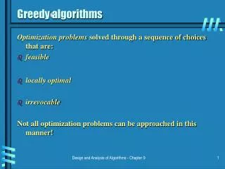
Why greedy algorithms? • Greedy algorithms are simple, and have efficient implementations • They are used as: • Exact algorithms for many optimization problems • Approximation schemes with guaranteed approximation ratios for hard problems • As heuristics for hard optimization problems
Goal To design an abstract model of greedy algorithms and answer the questions: • Could a known greedy approximation algorithm be improved? • Can we prove lower bounds on approximation ratio of greedy algorithms for hard problems? • Can we formalize the intuition that greedy algorithms are weaker than other algorithmic paradigms?
History • [BNR02] defined Priority algorithm framework for scheduling problems • [AB02] defined Priority algorithms for facility location and set cover • [BL03] proved bounds on performance of Priority algorithms for VC, IS and Coloring
General results • Extended the work of [BNR02] and [AB02] and defined problem-independent model for greedy algorithms • Defined a formal model of Memoryless priority algorithms • Characterization of the power of Fixed, Memoryless, and Adaptive algorithms in terms of combinatorial games
Separations Fixed Priority Algorithms Adaptive Priority Algorithms Dynamic Programming Algorithms Memoryless Priority Algorithms
Results for specific graph problems Shortest paths • No Fixed priority algorithm can achieve any constant approximation ratio, for ShortPath problem on graphs, with non-negative weights • No Adaptive priority algorithm can achieve any constant approximation ratio, for ShortPath problem on graphs with negative weights, but no negaitve weight cycles
Results for specific graph problems Steiner trees • Proved lower bound of 1.18 on the approximation ratio achieved by Adaptive priority algorithms • Improved adaptive priority algorithm, achieving an approximation ratio 1.875 for special metric instances where the distance between nodes is [1,2]
Results for specific graph problems Weighted Vertex Cover • Proved lower bound 2 for Adaptive priority algorithms, matching the standard 2-approximation scheme Independent Set • Proved lower bound of 3/2 on the performance of Adaptive algorithms for degree-3 graphs
Fixed Priority Algorithms Adaptive Priority Algorithms Remainder of the talk • What is a greedy algorithm? • Formal definitions of Fixed and Adaptive priority algorithms and show a strong separation between Fixed and Adaptive priority algorithms • Lower bound 2 on the approximation ratio of Adaptive priority algorithms on weighted vertex cover problem
What is a greedy algorithm? Given a universe of data items • The instance is a set of data items, subset of • The algorithm defines an ordering function on and views the data items in the instance in that order • The algorithm makes an irrevocable decision for each data item, which depends only on data items seen so far, and decisions made so far, not future data items • The solution is decisions made on each data item
Kruskal algorithm for MST Input (G=(V,E), ω: E →R) • Initialize empty solution T • L = Sorted list of edges in non-decreasing order according to their weight • while (L is not empty) • e = next edge in L • Add the edge to T, as long as T remains a forest and remove e from L • Output T
Fixed priority algorithms is a set of data items; is a set of options Input: instance I={1 ,2 ,…,n }, I Output: solution S={(i ,i) | i= 1,2,…,d}; i 1. Determine an ordering function π: →R+ {∞} 2. Order I according to π() 3. Repeat • Let the next data item in the ordering π be i • Make a decision i • Update the partial solution S until (decisions are made for all data items) 4. Output S={(i ,i) | i= 1,2,…,d}
Kruskal is a Fixed priority algorithm • is a set of edges • Each edge is represented as (u, v, ω) • ={accepted, rejected} • Priority function π: (u, v, ω)= ω
ShortPath ? Fixed Priority Algorithms Question: • Can all problems with known greedy algorithms be solved by a Fixed priority algorithm? ShortPath Problem: Given a graph G=(V,E), ω: E →R+; s, t V. Find a directed tree of edges, rooted at s, such that the combined weight of the path from s to t is minimal
ShortPath Answer: Fixed Priority Algorithms • Theorem: No Fixed priority algorithm can achieve any constant approximation ratio for the ShortPath problem
Solver Adversary Γ0 γd γ1 γ2 γ3 γi γj γk Solver is awarded Fixed priority game Γ0 Γ1 γi1 γi2 Γ2 γi3 γi4 γi5 Γ3 γi6 =∅ γi7 γi8 γi9,… σi2 σi4 End Game S_adv = {(γi2,σ*i2), (γi4,σ*i4)} S_sol = {(γi2,σi2)} S_sol = {(γi2,σi2), (γi4,σi4)}
Fixed priority game for ShortPath problem • Data items are edges of the graph • Decision options = {accept, reject} • A strategy for the Adversary in the game establishes a lower bound on approximation ratio achieved by any Fixed priority algorithm
u(k) a y(1) v(1) s t z(1) x(1) b w(k) Adversary selects 0
v(1) w(k) Solver selects an order on 0 If then the Adversary presents: u(k) a y(1) s t x(1) z(1) b
Event 1 σy=accept Event 2 σy=reject Adversary’s strategy Waits until Solver considers edge y(1) Solver will consider y(1) before z(1)
u(k) a y(1) t s z(1) x(1) b The Solver constructs a path {u,y} The Adversary outputs solution {x,z} Event 1: Solver accepts y(1)
z(1) Event 2: Solver rejects y(1) u(k) a y(1) t s x(1) b The Solver fails to construct a path. The Adversary outputs a solution {u,y}.
The outcome of the game: • The Solver either fails to output a solution or achieves an approximation ratio (k+1)/2 • The Adversary can set k arbitrarily large and thus can force the Algorithm to claim arbitrarily large approximation ratio
Conclusion • No Fixed priority algorithm can achieve any constant approximation ratio for the ShortPath problem • Dijkstra algorithm solves the ShortPath problem exactly Dijkstra algorithm (G=(V,E), s V) T←∅; S←{s}; Until (S≠V) • Find e=(u,x) | e = mineCut(S, V-S){path(s, x)+ω(e)} • T← T{e}; S ← S {x}
Adaptive priority algorithms is a set of data items; is a set of options Input: instance I={1, 2,…,d }, I Output: solution S={(i ,i) | i= 1, 2,…,d} 1. Initialization U=∅; S=∅;I*=∅;t=1 2. Repeat • Determine an ordering function πt: -I*→R+{∞} • Pick the highest priority data item tU according to πt • Make an irrevocable decision t • Update U ← U-{t}; S←S {(t,t)}; I*←I* {t}; t←t+1 until (decisions are made for all data items) 3. Output S={(i ,i) | i= 1,2,…,d}
ShortPath Adaptive Priority Fixed Priority Fixed Priority Algorithms Adaptive Priority Algorithms • Dijkstra is an Adaptive priority algorithm • is a set of edges;Each edge is represented as (u, v, ω) • ={accepted, rejected} • ordering
Weighted Vertex Cover • [Joh74] gave a greedy 2-approximation algorithm • Can we design an improved approximation algorithm in the class of Adaptive priority algorithms?
[Joh74] greedy 2-approximation for WVC Input: instance I={1, 2,…,n } Output: solution S I 1. Initialization U=∅; S=∅;I*=∅;t=1 2. Repeat • πt () = ω(v)/(|adj_list – I*|) • Order all tU according to their πt value in non-decreasing order. Let t be first data item in the order. • if (πt () ≠ ∞) then • Make an irrevocable decision t = in • Update U ← U-{t}; S←S {t}; I*←I* {t}; t←t+1 until (πt () ≠ ∞) 3. Output S
Priority model for WVC problem • A data item is a vertex of the graph = (v, ω(v), [adj_list] ); ω:V →R • The input to the algorithm is a set of data items I={1, 2,…,n} • Set of decision options is Σ={accept, reject} • Ordering function: πt () = ω(v)/(|adj_list – I*|) • For simplicity, the solution will be a vertex cover S I, of vertices accepted by the algorithm.
Question Is there an Adaptive priority algorithm which gives a better for the WVC than the known 2-approximation? –No! Theorem: No Adaptive priority algorithm can achieve an approximation ration better than 2
Solver Adversary Adaptive priority game Γ3 Γ1 Γ2 Γ0 γ9 γ10 γ12 γ2 γ3 γ7 γ6 γ8 γ5 γ11 γ1 γ4 S_sol = {(γ7,σ7), (γ4,σ4)} S_sol = {(γ7,σ7)} σ7 σ4 σ2 S_sol = {(γ7,σ7), (γ4,σ4),(γ2,σ2)} • The Game Ends: • S_adv = {(γ7,σ*7), (γ4,σ*4),(γ2,σ*2)} • Solver is awarded payoff • f(S_sol)/f(S_adv)
n2 n2 1 1 1 n2 n2 1 The Adversary chooses instances to be graphs Kn,n The weight function ω:V→ {1, n2}
The game • Data items • each node appears in oas two separate data items with weights 1, n2 • Solver moves • Choses a data item, and commits to a decision • Adversary move • Removes from the next t the data item, corresponding to the node just committed and..
1 1 1 1 1 Adversary’s strategy is to wait unitl Event 1: Solver accepts a node of weight n2 Event 2: Solver rejects a node of any weight Event 3: Solver has committed to all but one nodes on either side of the bipartite
n2 1 Event 1: Solver accepts a node ω(v)=n2 1 1 1 1 1 The Adversary chooses part B of the bipartite as a cover, and incurs cost n The cost of a cover for the Solver is at least n2+n-1
Event 2: Solver rejects a node of any weight n2 n2 The Adversary chooses part A of the bipartite as a cover. The Solver must choose part B of the bipartite as a cover.
1 Event 3: Solver commits to n-1 nodes w(v)=1, on either side of Kn,n 1 1 1 1 1 n2 1 The Adversary chooses part B of the bipartite as a cover, and incurs cost n The cost of a cover for the Solver is 2n-1
Summary • No Adaptive priority algorithm can achieve an approximation ratio better than 2 for the WVC • The known 2-approximation is optimal and cannot be improved
Fixed Priority Algorithms Adaptive Priority Algorithms Conclusions • The class of Adaptive priority algorithms is more powerful • The known 2-approximation for the WVC is optimal in the class of Adaptive priority algorithms and cannot be improved
Future research directions • Extend the framework to capture larger class of greedy algorithms • Define a notion of global information • Redefine the notion of local information • Build formal models for backtracking and dynamic programming algorithms and evaluate their performance on hard problems