Download
1 / 37
380 likes | 539 Views
Time Resolved Two Photon Photon-emission Diagnostic Technology and Data Acquisition. Bin Li. April. 7th, 2003. Mach Zehnder Interferometer. Piezo system. 2PPE UHV Chamber. Large fix time delay. Beam - splitter. Small fix time delay. SHG and Dispersion compensation.

E N D
Time Resolved Two Photon Photon-emission Diagnostic Technology and Data Acquisition Bin Li April. 7th, 2003
Mach Zehnder Interferometer Piezo system 2PPE UHV Chamber Large fix time delay Beam - splitter Small fix time delay SHG and Dispersion compensation Monochromator
Time Information and Alignment of Optics Monochromator N=2 N=1 N=0 L when we can get the first order of diffraction Pattern at Grating d Select a single wavelength out of the femto-second laser’s wave package.
Our pulsed laser repetition rate is 83MHz, repetition time period is around 0.012 us, which is much faster than the response time of photo-diode detector. So we can treat the two different components as continuous wave. Output is coherent interference signal of these two split beams:
The Delayed time can be generated by using scanning signal of piezo -system, one arm fixed, the other arm moves to a distance: Good Bad So we can get the precise time delay between two beams from this signal; meanwhile, we also can see if the optics alignment in MZI is good or not.
Dispersion Compensation After traveling finite distance In air or optics, the different components of femto–second pulse will arrive at different time! T In order to make different wavelets in a same phase, we have to generate negative dispersion! One widely used method: Multiple Coating Reflection Mirror, the deeper layers have smaller index.
A simple calculation: Two Layers Case Where n1>n2 n2 So when Evanescent wave n1 There should be TIR, but when the medium is thin, we have penetration depth: n0 Air Optical Length path: Negative Dispersion !!
In Our Experiment, we combine the discrete negative dispersion (Chirp Mirror) with continuous positive dispersion (Wedge). But how do we know when the minimal dispersion occurs? We do need another diagnostic signal to indicate the dispersion!! Intensity Spectrum When pump pulse and probe pulse are orthogonal polarization, we have Intensity cross-correlation: No phase information! Interference Signal The case when they have same polarization:
So we have: , are average intensity of Beam 1 and Beam 2, they are constant. And Let’s consider the Fourier transformation:
When the two output beams are identical, we just get the spectral intensity of light: For Gaussian pulse Fourier Transformation is Since the first order Interference signal has high background (peak to background ratio is 2:1), people are not using it as an indicator of phase or dispersion. Instead, we use SSHG. Sample p-Polarization x s-Polarization Electron Photoemission Selection Filter
The filter will eliminate the fundamental, the second order interferometric correlation signal will be detected: By using We get: where
Considering Identical fields case: When time delay , we will get the sum of all constructive interference terms: When time delay is large, the cross product terms vanish, so we have a background value: The peak to background ratio is 8:1, and it is sensitive to the pulse phase modulation, so people use it as diagnostic signal for quantitatively measur -ement of linear chirp!! (Jean-Claude Diels, Wolfgang Rudolph, Ultrashort Laser Pulse Phenomena, Academic Press, 1996)
More discussion on dispersion Taylor Expansion at center frequency : (L is the optical length in Air or Optics.) Just consider up to 1st order , in frequency region: In time Region:
After rearrangement, we obtain: Up to 1st order expansion of wave number k is just a time delay factor: By using We get
GVD (Group Velocity Dispersion) for Gaussian Pulse Bring in the GVD term and neglect the Time Delay Factor: For femto second Laser source, under equal mode approximation, we get In real case, the laser amplification profile will make each mode has different amplitude, in order to make calculation simpler, it is good to use Gaussian Approximation:
By the way, If we use repetition rate: and the pulse width: (The number of Mode Locking is in the order of million !!) We can compare these two normalized functions, they are pretty close. Gaussian Shape is a fairly good Approximation.
So we will get: When GVD is a small value , we have: Conclusion: GVD term is the linear chirp of Gaussian Pulse. Here we can see linear chirp:
Previously, we have second order interferometric signal: If we consider a linearly chirped Gaussian pulse: There will be: Let Optical cycle and pulse width By using linear chirp term: a1=0.1, a2=0.5, a3=2, a4=4, a5=16, we will get the following second harmonic interferometric correlation signal!
So from this signal, we can minimize the GVD, meanwhile we can estimate the pulse width of our femto second Laser.
Evac 2 ECBM 1 Ef 0 EVBM Time Resolved Interferometric 2PPE Correlation Ultrafast interferometric pump-probe techniques can be applied to metals or semiconductors, decay rates of hot-electron population and quantum phase and other underlying dynamics can be extracted by careful analysis the 2PPE Signal. Ev Ef Metal Semi-conductor T1 population relaxation time, T2 coherence decay time.
Quantum Perturbation Theory (First Order Approximation) Before Apply pump-probe laser pulse, electrons are in non-interacting discrete Energy Levels: After introducing laser pulses, Hamiltonian becomes: Let Put it in We have Multiplied by , then do integration, using the orthonormal condition.
So where and Using real electric field: Assuming small dispersion, chirp term disappears ! Now For Bosonic system, we have For Fermionic system, we have
Hot electronic energy states is in a Fermionic system, and we consider the case The laser energy is just good for the transitions: between an initial energy state, which is below the Fermi energy and an intermediate energy state, which is an excited state above Fermi level, or between an intermediate energy state and a Final state, which is above the Vacuum level and can be observed by Energy Analyzer. E2 Ev Eint Ef E1 Absorbing the constant factor into amplitude (here we can use Gaussian Approximation), considering just one dimensional dipole transition, the pump-probe perturbation term becomes:
So for electrical dipole moment operator , only two adjacent terms do not vanish at certain constrains! Here, I just do a simple calculation for dipole transition term; in fact, the more accurate results rely on the knowledge of the interacting quantum states of the system and the polarization of the electric field. For example, transition from to The transition term should be:
So, for a three-Level-Atom-System, with pump-probe radiation perturbation, we have: Let Estimate (Detuning of resonance) By using initial condition: and integration recurrently, Theoretically, We can solve the derivative equation and get C0(t), C1(t), C2(t)
Now we discuss the density operators, which are measurable quantities, and we can compare them with the 2nd order auto-correlation signal, then extract useful dynamics out of them. Each component has: Now we can calculate the 1st order derivative equations of , but we have to consider one more thing. Since level 1 and level 2 are above the Fermi levels, are unoccupied states, so their population densities will relax to zero quickly, meanwhile we have to consider the coherent decay between different polarizations induced by one photon pulse excitation or two-photon excitation . Where we define as population relaxation time of level 1 and level 2; as 1st order decoherent time, and as 2nd order decoherent time. Then, we will get 9 first order derivative equations for population density (when m=n, diagonal terms), or coherence dynamics (when m!=n, off-diagonal elements).
Since only the energy of Level 2 is above the vacuum level, so the time resolved 2PPE correlation signal is the dynamics of . Not just , but the average value of it. Here laser pulse is 10 femto-second, Energy Analyzer acquisition time is about 163.84 us, pulse repetition time is about 0.012 us, so our detected 2PPE signal is including about 13,500 different pump-probe coherent interacting processes with electrons. The signal amplitude is mainly dependent on the delay time between pump and probe pulses ------ , the relaxation time ----- T1 , and coherent time T2. From Set By using
So, we get And the measured electron photon-emission signal can be denoted as: It only depends on the delay time between two pulses. How can we solve the derivative function of ? Firstly, we have to consider By using:
and So finally, we will get: We see solving derivative equation of is not the end of story, it depends on other variables, such as So we can expect these nine elements of density matrix are dependent on each others, they only way to get the absolute solution for is to solve all these 6 dependent derivative equations (some of them are complex conjugates). We can plug in reasonable parameters and solve those equations to see how well the theoretic calculation match with real time experimental results !!!
Another Process: Fitting Procedure for the calculation of the relaxation time and decoherent time: [W. Nessler, S. Ogawa, H. Nagano, H. Petek, etc, J. of Elec. Spec and Phenomena, 88-91 (1998) 495] Simulation of TR-2PPE process by using Perturbation Theory is entangled Quite a few unknown quantities together, it is not easy to extract information from it, so there is a consideration from another point of view. From previous discussion, we know the 2nd order interferometric signal of the Gaussian pulse with negligible dispersion is: It includes 0w (phase averaged component), 1w (1st order component), and 2w (2nd order component).
For Gaussian pulse , The 0w,1w, and 2w components have time respectively. So, same as SSHG, the pump-probe electron emission will have similar signal, but more. The same is the two pulse or two induced polarization interference, the additional part is the response of electron (coherent interaction, population relaxation). Now if we think the first laser pulse excites the electron to intermediate level, then the 2nd pulse just works as a probe to get the dynamics of the intermediate Energy level. So the 0w, 1w and 2w components should be convolution between Pulsed signal and the coherent decay or in coherent decay. , where Is the FWHM of Gaussian Pulse. If you still want to use the notation of , we have the identical convolution:
0w (Phase Average Component) consists both coherent parts and incoherent, and background term, so: Fitting these three theoretical calculated curves with Fourier Transformation (2w, 1w, 0w) of experimental 2PPE correlation signal respectively, we can get the population decay time , decoherent time of first order , and 2nd order of intermediate level of our system. The following are Fourier Transformation terms:
Apply this fitting procedure to TR-2PPE Signal
200 TiO2 Clean Surface at 110K 150 1:(5.8 eV) 2PPE Intensity (CPS) 100 2:(5.71 eV) 3:(5.9 eV) 5:(6.01 eV) 50 7:(6.12 eV) 0 5.0 5.2 5.4 5.6 5.8 6.0 6.2 6.4 6.6 6.8 7.0 Hot Electron Final Energy (eV) Our Experiment Data on TiO2 (110) surface Example Clean Surface 7-Channel Data Acquisition & Time-resolved Measurement
raw data phase average 1w envelope 2w envelope T1(1) : 19.5 fs 1.0 0.8 T2(01): 5.2 fs 0.6 intensity [normalized] T2(02): 1.8 fs 0.4 0.2 0.0 -50 0 50 100 150 Time delay [fs]
Hot Electron Relaxation Time --- T1 25 20 15 Time (fs) 10 5 0 2.4 2.5 2.6 2.7 2.8 2.9 3 Intermediate State Energy Level (eV) The Relaxation Time is pretty close to a constant (around 20 femto-seconds! )