Download
1 / 66
740 likes | 1.07k Views
ISAPP 2011, International School on Astroparticle Physics 26 th July–5 th August 2011, Varenna, Italy. Neutrinos from the Sun. Neutrinos and the Stars II Neutrinos from the Sun. Georg G. Raffelt Max-Planck-Institut f ür Physik, München, Germany. Neutrinos from the Sun. Helium.

E N D
ISAPP 2011, International School on Astroparticle Physics 26th July–5th August 2011, Varenna, Italy Neutrinos from the Sun Neutrinos and the Stars II Neutrinos from the Sun Georg G. Raffelt Max-Planck-Institut für Physik, München, Germany
Neutrinos from the Sun Helium Reaction- chains Energy 26.7 MeV Solar radiation: 98 % light 2 % neutrinos At Earth 66 billion neutrinos/cm2 sec Hans Bethe (1906-2005, Nobel prize 1967) Thermonuclear reaction chains (1938)
Hydrogen Burning: Proton-Proton Chains < 0.420 MeV 1.442 MeV 100% 0.24% 85% 15% PP-I hep < 18.8 MeV 90% 10% 0.02% 0.862 MeV 0.384 MeV < 15 MeV PP-II PP-III
Proposing the First Solar Neutrino Experiment John Bahcall 1934 – 2005 Raymond Davis Jr. 1914 –2006
First Measurement of Solar Neutrinos Inverse beta decay of chlorine 600 tons of Perchloroethylene Homestake solar neutrino observatory (1967–2002)
Results of Chlorine Experiment (Homestake) ApJ 496:505, 1998 Average Rate Average (1970-1994)2.56 0.16stat 0.16sysSNU (SNU = Solar Neutrino Unit = 1 Absorption / sec / 1036 Atoms) Theoretical Prediction 6-9 SNU “Solar Neutrino Problem” since 1968
Neutrino Flavor Oscillations Two-flavor mixing Each mass eigenstate propagates as with Phase difference implies flavor oscillations Probability Bruno Pontecorvo (1913–1993) Invented nu oscillations z Oscillation Length
GALLEX/GNO and SAGE Inverse Beta Decay Gallium Germanium GALLEX/GNO (1991–2003)
Cherenkov Effect Light Electron or Muon (Charged Particle) Neutrino Light Cherenkov Ring Elastic scattering or CC reaction Water
Super-Kamiokande Neutrino Detector (Since 1996) 42 m 39.3 m
Sudbury Neutrino Observatory (SNO) 1000 tons of heavy water
Sudbury Neutrino Observatory (SNO) 1000 tons of heavy water
Sudbury Neutrino Observatory (SNO) 1000 tons of heavy water Normal (light) water H20 Heavy water D20 Nucleus of hydrogen (proton) Nucleus of heavy hydrogen (deuterium)
Sudbury Neutrino Observatory (SNO) Heavy hydrogen (deuterium) Heavy hydrogen (deuterium) Electron neutrinos All neutrino flavors
Missing Neutrinos from the Sun All Flavors Water Water Heavy Water Heavy Water Chlorine Gallium ne+e- ne+e- n+ e- n+ e- ne+dp+p+e- n+dp+n+n 8B 8B 8B 8B 8B 8B CNO 7Be pp CNO 7Be Homestake Gallex/GNO SAGE (Super-) Kamiokande SNO SNO Electron-Neutrino Detectors
Charged and Neutral-Current SNO Measurements Ahmad et al. (SNO Collaboration), PRL 89:011301,2002 (nucl-ex/0204008)
Final SNO Measurement of Boron-8 Flux SNO Collaboration, arXiv:0910.2984
KamLAND Long-Baseline Reactor-Neutrino Experiment • Japanese Nuclear Reactors • 80 GW (20% world capacity) • Average distance 180 km • Flux 6 105cm-2s-1 • Without oscillations • 2 captures per day
Oscillation of Reactor Neutrinos at KamLAND (Japan) Oscillation pattern for anti-electron neutrinos from Japanese power reactors as a function of L/E KamLAND Scintillator detector (1000 t)
Solar Neutrino Spectrum 7-Be line measured by Borexino (2007)
Solar Neutrino Spectroscopy with BOREXINO • Neutrino electron scattering • Liquid scintillator technology • ( 300 tons) • Low energy threshold • ( 60 keV) • Online since 16 May 2007 • Expected without flavor oscillations • 75 ± 4 counts/100 t/d • Expected with oscillations • 49 ± 4 counts/100 t/d • BOREXINO result (May 2008) • 49 ± 3stat ± 4syscnts/100 t/d • arXiv:0805.3843 (25 May 2008)
Solar Neutrinos in Borexino Borexino Collaboration, arXiv:1104.1816
Geo Neutrinos Geo Neutrinos
Geo Neutrinos: What is it all about? • We know surprisingly little about • the Earth’s interior • Deepest drill hole 12 km • Samples of crust for chemical • analysis available (e.g. vulcanoes) • Reconstructed density profile • from seismic measurements • Heat flux from measured • temperature gradient 30-44 TW • (Expectation from canonical BSE • model 19 TW from crust and • mantle, nothing from core) • Neutrinos escape unscathed • Carry information about chemical composition, radioactive energy • production or even a hypothetical reactor in the Earth’s core
Geo Neutrinos Expected Geoneutrino Flux KamLAND Scintillator-Detector (1000 t) Reactor Background
Latest KamLAND Measurements of Geo Neutrinos K. Inoue at Neutrino 2010
Geo Neutrinos in Borexino Geo neutrino signal Borexino Collaboration, arXiv:1003.0284v
Geo Neutrinos in Borexino Expectation Reactors 99.73% 95% 68% Expectation BSE model of Earth Borexino Collaboration, arXiv:1003.0284
Solar Models Solar Models
Equations of Stellar Structure Assume spherical symmetry and static structure (neglect kinetic energy) Excludes: Rotation, convection, magnetic fields, supernova-dynamics, … • Hydrostatic equilibrium • Energy conservation • Energy transfer • Literature • Clayton: Principles of stellar evolution and • nucleosynthesis (Univ. Chicago Press 1968) • Kippenhahn & Weigert: Stellar structure • and evolution (Springer 1990) Radius from center Pressure Newton’s constant Mass density Integrated mass up to r Luminosity (energy flux) Local rate of energy generation Opacity Radiative opacity Electron conduction
Convection in Main-Sequence Stars Sun Kippenhahn & Weigert, Stellar Structure and Evolution
Constructing a Solar Model: Fixed Inputs Solve stellar structure equations with good microphysics, starting from a zero-age main-sequence model (chemically homogeneous star) to present age Adapted from A. Serenelli’s lectures at Scottish Universities Summer School in Physics 2006
Constructing a Solar Model: Free Parameters • 3 free parameters • Convection theory has 1 free parameter: • Mixing length parameter aMLT • determines the temperature stratification where convection • is not adiabatic (upper layers of solar envelope) • 2 of the 3 quantities determining the initial composition: • Xini, Yini, Zini(linked by Xini + Yini + Zini = 1). • Individual elements grouped in Zini have relative abundances • given by solar abundance measurements (e.g. GS98, AGSS09) • Construct a 1 M⊙initial model with Xini, Zini, Yini = 1 - Xini - Zini and aMLT • Evolve it for the solar age t⊙ • Match (Z/X)⊙, L⊙ and R⊙ to better than one part in 105 Adapted from A. Serenelli’s lectures at Scottish Universities Summer School in Physics 2006
Standard Solar Model Output Information Eight neutrino fluxes: Production profiles and integrated values. Only 8B flux directly measured (SNO) • Chemical profiles X(r), Y(r), Zi(r) • electron and neutron density profiles (needed for matter effects in neutrino studies) Thermodynamic quantities as a function of radius: T, P, density (r), sound speed (c) Surface helium abundance Ysurf (Z/X and 1 = X + Y + Z leave 1 degree of freedom) Depth of the convective envelope, RCZ Adapted from A. Serenelli’s lectures at Scottish Universities Summer School in Physics 2006
Solar Models Helioseismology and the New Opacity Problem
Helioseismology: Sun as a Pulsating Star • Discovery of oscillations: Leighton et al. (1962) • Sun oscillates in > 105 eigenmodes • Frequencies of order mHz (5-min oscillations) • Individual modes characterized by • radial n, angular l and longitudinal m numbers Adapted from A. Serenelli’s lectures at Scottish Universities Summer School in Physics 2006
Helioseismology: p-Modes • Solar oscillations are acoustic waves • (p-modes, pressure is the restoring force) • stochastically excited by convective motions • Outer turning-point located close to temperature inversion layer • Inner turning-point varies, strongly depends on l (centrifugal barrier) Credit: Jørgen Christensen-Dalsgaard
Examples for Solar Oscillations + + = http://astro.phys.au.dk/helio_outreach/english/
Helioseismology: Observations • Doppler observations of spectral • lines measure velocities of a few cm/s • Differences in the frequencies • of order mHz • Very long observations needed. • BiSON network (low-l modes) • has data for 5000 days • Relative accuracy in frequencies is 10-5
Helioseismology: Comparison with Solar Models • Oscillation frequencies depend on r, P, g, c • Inversion problem: • From measured frequencies and from a reference solar model • determine solar structure • Output of inversion procedure: dc2(r), dr(r), RCZ, YSURF Relative sound-speed difference between helioseismological model and standard solar model
New Solar Opacities (Asplund, et al. 2005, 2009) • Large change in solar composition: • Mostly reduction in C, N, O, Ne • Results presented in many papers by the “Asplund group” • Summarized in Asplund, Grevesse, Sauval & Scott (2009) Adapted from A. Serenelli’s lectures at Scottish Universities Summer School in Physics 2006
Origin of Changes • Improved modeling • 3D model atmospheres • MHD equations solved • NLTE effects accounted for in most cases • Improved data • Better selection of spectral lines • Previous sets had blended lines • (e.g. oxygen line blended with nickel line) Spectral lines from solar photosphere and corona Meteorites • Volatile elements • do not aggregate easily into solid bodies • e.g. C, N, O, Ne, Ar only in solar spectrum • Refractory elements • e.g. Mg, Si, S, Fe, Ni • both in solar spectrum and meteorites • meteoritic measurements more robust
Consequences of New Element Abundances What is good • Much improved modeling • Different lines of same element give • same abundance (e.g. CO and CH lines) • Sun has now similar composition • to solar neighborhood New problems • Agreement between helioseismology • and SSM very much degraded • Was previous agreement a coincidence? Adapted from A. Serenelli’s lectures at Scottish Universities Summer School in Physics 2006
Standard Solar Model 2005: Old and New Opacity Sound Speed Density Adapted from A. Serenelli’s lectures at Scottish Universities Summer School in Physics 2006