Download
1 / 34
420 likes | 1.01k Views
Interconnection Networks in Multiprocessor Systems. By: Wallun Chan Course: CS 147 Text: Chapter 12, p. 528 - 539 Professor: Sin-Min Lee. Table of Contents. Introduction Fixed Connections Examples of some fixed communication connection systems Clustered communication system

E N D
Interconnection Networks in Multiprocessor Systems By: Wallun Chan Course: CS 147 Text: Chapter 12, p. 528 - 539 Professor: Sin-Min Lee
Table of Contents • Introduction • Fixed Connections • Examples of some fixed communication connection systems • Clustered communication system • Reconfigurable communication connections • Crossbar switch system • Multistage interconnection networks (MIN) • Generalized Clos network • Example of the Benes network • Example of the Omega network • Example of the Baseline network • Routing on Multistage Interconnection Networks • Example of a routing algorithm for Benes network • Example of a routing algorithm for Omega network • Switching techniques • Store-and-forward • Circuit switching • Virtual cut-through switching • Wormhole routing
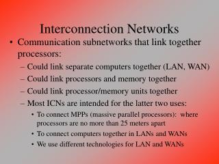
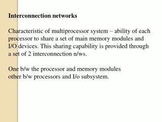
Introduction • What are interconnection networks and why are they important? • Processors in a parallel computer need to communicate in order to solve a problem. Therefore, there is a need for some kind of communication highway or interconnection network, i.e. the processors to be connected in some pattern. • Performance in multiprocessor systems are highly dependent on communication processes between processors and memory, I/O devices, and other processors. Therefore, choosing the right interconnection network is important for efficiency reasons. • Interconnection networks can be categorized according to criteria such as topology, routing strategies, and switching techniques. • Topology is the pattern in which the individual processors are connected to other elements. The two main topologies are fixed and reconfigurable. • Routing strategies are procedures used to set switches and plays a crucial role in the performance of multistage interconnection networks • Switching techniques are ways that data packets are handled on their way from a source to a destination processor.
Fixed Interconnection Networks • Fixed connection systems are hard-wired in place and cannot change their configurations. • Although not as flexible as reconfigurable connection systems, they are sufficient for most parallel computing demands and are less costly. • Generally, fixed topologies are suited for problems with well predicted communication patterns. • Mainly used for message-passing architectures. • Some examples of fixed connections include: • One fixed connection topology not discussed so far: • Clustered fixed connection
Some Multiple Instruction Multiple Data (MIMD) Fixed Connections M M M P ... P P P P P Cluster bus P P Global memory P A) Shared bus B) Ring P P P P P P P P P P P P P P P P C) Tree D) Mesh
P P P P P P P P P P P P P P P P P P P P P P P P E) Hypercube F) Completely connected Other MIMD Fixed Connections BACK
P P P P Intercluster gateway P Intercluster gateway P Cluster bus Cluster bus P P P P P P P P P P Intercluster gateway Intercluster gateway Cluster bus Cluster bus P P P P Clustered 16-Processor Fixed Connection • Divided into 4 clusters. • 4 processors per cluster connected by cluster bus. P P P P P • 2 processors in same cluster bus can communicate with each other without affecting other clusters; this maximizes data flow and minimizes delay. Intercluster gateway Intercluster gateway Intercluster gateway Intercluster gateway Cluster bus Cluster bus Cluster bus Cluster bus P P P P P Intercluster communications mechanism Intercluster communications mechanism • Intercluster gateways allow transfers between clusters. P P P P • The intercluster communications mechanism communicates between clusters; this may be a fixed or reconfigurable network. Intercluster gateway Intercluster gateway Intercluster gateway Intercluster gateway Cluster bus Cluster bus • If a task requires processors in more than one cluster, the following process occurs. P P P P
Cluster to Cluster Communication in 16-processor Fixed Connection • A processor in one cluster sends data and destination information to its intercluster gateway via its cluster bus. P P P P P Intercluster gateway Intercluster gateway Intercluster gateway • The gateway evaluates the destination information to find its cluster. Cluster bus Cluster bus Cluster bus P P P P • The data is then sent to the specified cluster through the communications mechanism. Intercluster communications mechanism Intercluster communications mechanism P P P P • Finally, the destination gateway sends the data to the destination processor. Intercluster gateway Intercluster gateway Intercluster gateway Cluster bus Cluster bus Cluster bus • The processors never talk to each other directly; processors are free while gateways send the data. P P P P P
Reconfigurable Connections • When different tasks require different processing resources, reconfigurable connections are needed. • Reconfigurable connections allow for dynamic configurations to match individual tasks thereby optimizing overall system performance. • Several reconfigurable connection configurations exist • Crossbar switch connections • Multistage interconnection networks (MINs)
0 1 inputs . . . . . . n - 1 0 1 m - 1 ... outputs Crossbar Switch Connections • Has n inputs and m outputs; n and m are usually the same. • Data can flow in either directions. • Each crosspoint can open or close to realize a connection. • All possible combinations can be realized. • The inputs are usually connected to processors and outputs connected to memory, I/O, or other processors. • These switches have complexities of O(n2); doubling the number of inputs and outputs also doubles the size of the switch. • To solve this problem, multistage interconnection networks were developed.
0 0 0 0 1 1 1 1 Straight Exchange Multistage Interconnection Networks • Use smaller crossbar switches, usually 2 x 2, connected by fixed links. • These 2 x 2 switches have 2 possible settings for permutation networks, straight and exchange, as shown in figures below. • Inputs and outputs are connected in a 1 to 1 manner. • Multistage interconnection networks realize desired permutation networks of their inputs and outputs by setting the switches to the correct states. • Routing algorithms are used to set the switches of a multistage interconnection network.
Permutation Networks • Most multistage interconnection networks are designed to realize permutation networks, that is, networks with 1 to 1 connections between their inputs and outputs. • Multistage interconnection networks are classified into 2 groups. • Nonblocking - can realize any of the n! connections between its n inputs and n outputs. • Strictly nonblocking - can change a connection without affecting any other connections. • Rearrangeably nonblocking - can realize new connections but may have to reroute existing connections. • Blocking - cannot realize every possible combination between its inputs and outputs. • Some widely used multistage interconnection networks include • Clos network • Benes network • Omega network • Baseline network
0 0 1 1 0 k - 1 k - 1 0 0 1 1 0 m - 1 n - 1 0 0 1 1 0 n - 1 m - 1 . . . . . . . . . . . . . . . . . . 0 0 1 1 1 k - 1 k - 1 0 0 1 1 1 m - 1 n - 1 0 0 1 1 1 n - 1 m - 1 . . . . . . . . . . . . . . . . . . 0 0 1 1 m - 1 k - 1 k - 1 0 0 1 1 k - 1 m - 1 n - 1 0 0 1 1 k - 1 n - 1 m - 1 . . . . . . . . . . . . . . . . . . Generalized Clos Network NEXT • 3 stages of switches with T = n * k inputs and outputs. inputs outputs • 1st stage has k switches of size n by m. 0 0 0 0 1 1 0 n - 1 m - 1 0 0 1 1 0 k - 1 k - 1 0 0 1 1 0 m - 1 n - 1 1 1 . . . . . . . . . . . . . . . . . . • 2nd stage has m k by k switches that receive 1 input from each 1st stage switch. n - 1 n - 1 n n • 3rd stage has k m by n switches that receive 1 input from each 2nd stage switch. 0 0 1 1 1 n - 1 m - 1 0 0 1 1 1 k - 1 k - 1 0 0 1 1 1 m - 1 n - 1 n + 1 n + 1 . . . . . . . . . . . . . . . . . . 2n + 1 2n + 1 • If m n, network is rearrangeably nonblocking. . . . . . . . . . • If m 2n-1, network is strictly nonblocking. T - n T - n 0 0 1 1 k - 1 n - 1 m - 1 0 0 1 1 m - 1 k - 1 k - 1 0 0 1 1 k - 1 m - 1 n - 1 T - n + 1 T - n + 1 . . . . . . . . . . . . . . . . . . • n, m, and k can be changed to realize complexities between O(n lg n) to O(n2). T - 1 T - 1
Benes Network • Derived from Clos network by setting n = m = 2, and k = T / 2, and recursively decomposing the two center (T / 2) x (T / 2) switches. BACK 0 0 1 1 • For example, to create an 8 x 8 Benes network, four 2 x 2 switches in the 1st and last stages are created. 2 2 • Two 4 x 4 switches in center stage. 3 3 • 1 output of each 1st stage switch routed to an input of each center stage switch. 4 4 • 1 input of each last stage switch routed from an output of each center stage switch. 5 5 • The center stage switches are further decomposed into 4 x 4 Benes networks. 6 6 7 7 • Is rearrangeably blocking and has complexity of O(n lg n).
E A I F B J G C K H D L 8 x 8 Omega Network • Consists of four 2 x 2 switches per stage. 0 0 • The fixed links between every pair of stages are identical. A E I 1 1 • A perfect shuffle is formed for the fixed links between every pair of stages. 2 2 B F J 3 3 4 4 • Has complexity of O(n lg n). C G K 5 5 • For 8 possible inputs, there are a total of 8! = 40,320 1 to 1 mappings of the inputs onto the outputs. But only 12 switches for a total of 212 = 4096 settings. Thus, network is blocking. 6 6 D H L 7 7
E I F K G J H L A 0 0 A 1 1 C 2 2 C 3 3 B 4 4 B 5 5 D 6 6 D 7 7 Baseline Network • Similar to the Omega network, essentially the front half of a Benes network. • The figure to the right shows an 8 x 8 Baseline network. • To generalize into an n x n Baseline network, first create one stage of (n / 2) 2 x 2 switches. • Then one output from each 2 x 2 switch is connected to an input of each (n / 2) x (n / 2) switch. • Then the (n / 2) x (n / 2) switches are replaced by (n / 2) x (n / 2) Baseline networks constructed in the same way. • The Baseline and Omega networks are isomorphic with each other.
0 0 E I A 1 1 2 2 C G J 3 3 4 4 B F K B F J 5 5 6 6 H L D C G K 7 7 Isomorphism Between Baseline and Omega Networks (cont.) • Starting with the Baseline network. • If B and C, and F and G are repositioned while keeping the fixed links as the switches are moved. • The Baseline network transforms into the Omega network. • Therefore, the Baseline and Omega networks are isomorphic.
Routing on Multistage Interconnection Networks • Routing algorithms play a crucial role in the performance of a multistage interconnection network. Slow routing algorithms will greatly reduce the performance of a multiprocessor system. • A multistage interconnection network can have many different routing algorithms from which to choose. But one is chosen and implemented into the system during its design. • But before examining routing algorithms for multistage interconnection networks, notations for permutations must be introduced.
01 10 01 01 01 01 01 10 . . , . 0 0 0 0 1 1 1 1 Straight Exchange Permutation Notation • A permutation is represented as a two-row matrix bounded by parentheses. The top row is the list of sources, and the bottom row is the list of destinations. • For example, the straight permutation of the switch below would be • represented as • The exchange permutation would be represented as • The group realizable by this switch is
0 0 1 1 2 2 3 3 4 4 0 1 0 1 2 3 3 2 4 5 5 4 6 7 6 7 5 5 , , , . 6 6 0 1 2 3 4 5 6 7 0 1 3 2 5 4 6 7 . 7 7 Permutation Notation (cont.) • Settings of individual switches of a stage can be concatenated to form settings for entire stages. • For example, in the Benes network, assume the switches in the 1st stage are set to realize • The setting for the entire stage is the concatenation of these settings,
0 1 0 0 1 1 2 3 2 2 4 3 3 5 4 4 6 5 5 0 1 2 3 4 5 6 7 0 4 1 5 2 6 3 7 0 1 2 3 4 5 6 7 0 4 5 1 6 2 3 7 0 1 2 3 4 5 6 7 0 1 3 2 5 4 6 7 . . . 7 6 6 7 7 i-1 p = (p(Sj) x Lj) x p(Si) j=1 Permutation Notation (cont.) • To express the mapping realized by sequential permutations, the permutations are combined. • For example, assume the 1st stage switches are set to realize p(S1) = • The links are fixed and always realize the mapping • So the result for the 2nd stage is p(S1) x L1 = • The permutation of a network can be expressed as the product of the stage and link permutations:
Looping Algorithm for Benes Network • This is a recursive method used to set the switches of a Benes network. • Recall that the Benes network is recursive in structure, consisting of two outer stages of switches and two half size Benes networks. • This algorithm takes advantage of the recursion as it sets the switches of the Benes network. • It takes the initial permutation, sets the switches in the outer stages, and generates the permutations to be realized by the two subnetworks. These permutations are processed recursively until the entire network is set. • The run time of this algorithm is O(n lg n). • Illustration
0 0 1 1 2 2 3 3 4 4 5 5 6 6 0 1 2 3 4 5 6 7 1 2 3 4 5 6 7 0 . 7 7 Looping Algorithm for Benes Network (cont.) • To illustrate, consider the 8 x8 Benes network that must realize the permutation • The algorithm starts by arbitrarily setting any one switch in an outer stage. • The uppermost switch in the 1st stage is set to straight and sends network input 0 to the upper subnetwork. • Each switch in last stage receives 1 input from upper subnetwork and 1 from lower subnetwork. • Since network input 0 is routed to upper subnetwork, and this input must be routed to network output 1, the uppermost switch in the last stage must be set to exchange. • Network output 0 then receives its data from the lower subnetwork. And since its source is network input 7, its switch is set to straight. This causes network input 6 to be routed to the upper subnetwork. If any switches in outer stages are not set, then one is arbitrarily set again. • This algorithm follows the same procedure, looping back and forth between inputs and outputs, until the original switch is reached.
0 1 0 0 2 1 1 3 4 5 6 2 2 1 3 3 7 0 0 2 4 6 1 3 5 7 1 3 5 7 2 4 6 0 3 and 4 4 2 5 5 5 respectively. 4 7 6 6 7 7 6 After 1 Iteration of Looping Algorithm • After the first iteration of the looping algorithm, the outer stage switches are set as shown in the figure to the right. • The permutation to be realized by the upper and lower subnetworks are
0 0 1 1 2 2 3 3 4 4 5 5 0 1 2 3 4 5 6 7 1 2 3 4 5 6 7 0 . 6 6 7 7 Final Results of Looping Algorithm • Repeating the algorithm on the subnetworks yields the final switch settings shown in the figure to the right according to the permutation
Routing Algorithm for Omega Network • Unlike the Benes network, which uses a centralized algorithm to set all of its switches, the Omega network uses a distributed, self routing procedure. • The switches examine the destinations of their input data and set themselves. No central routing hardware is needed. • Because of this, the switches in each stage can be set in parallel, and the network can be set up in O(lg n) time.
0 0 A E I 1 1 2 2 B F J 3 3 4 4 C G K 5 5 6 6 D H L 7 7 Routing Algorithm for Omega Network (cont.) • To understand this routing algorithm, consider the 1st stage of the Omega network to the right. E I • All four 1st stage switches send their upper outputs to switches E and G, and their lower outputs to switches F and H. F J • Switches E and G both send their outputs to switches I and J; their data can only reach the network outputs of 0, 1, 2, and 3. G K • Similarly, data from switches F and H can only reach network outputs 4, 5, 6, and 7. H L
0 0 A E I 1 1 2 2 B F J 3 3 4 4 C G K 5 5 6 6 D H L 7 7 Routing Algorithm for Omega Network (cont.) • Each 1st stage switch must be set so that its upper output has a destination with binary value 000, 001, 010, or 011, i.e. having 0 in the first bit position of its destination. BLOCKED (111) (100) (111) • Similarly, the lower output of each 1st stage switch must have a 1 in the first bit position of its destination to reach outputs 100, 101, 110, or 111. • For example, if network input 0 has to establish a connection with network output 7 (111), then the uppermost 1st stage switch must set itself to exchange. • If two inputs to a 1st stage switch have the same value in the first bit position, the Omega network cannot realize this permutation. • For example, if network input 0 has network output 4 and network input 1 has network output 7 as their destinations, then switch A is blocked since both 4 (100) and 7 (111) have bit 1 in their first bit position.
0 0 A E I 1 1 2 2 B F J 3 3 4 4 C G K 5 5 6 6 D H L 7 7 Routing Algorithm for Omega Network (cont.) • Similarly, the 2nd stage switch sends its upper output to switches I or K, which connect to outputs 0 (000), 1 (001), 4 (100), and 5 (101). I • The lower outputs can reach switches J or L, which can access outputs 2, 3, 6, and 7 (010, 011,110, and 111). J • For the second stage, the 2nd bit of the destination determines the setting of the switch. K • Similarly, the least significant bit of the destination determines the setting of the switches in the 3rd stage. L • Since the 3rd stage outputs are the outputs of the network, the last stage cannot block a permutation that has been routed successfully by the previous stages.
Successful Omega Routing Scheme 111 011 000 0 0 011 001 1 1 000 111 011 001 2 2 110 3 3 101 010 001 101 000 4 4 101 5 5 010 100 111 010 110 6 6 100 100 110 7 7
Unsuccessful Omega Routing Routing 100 000 0 0 BLOCK 000 1 1 001 100 101 2 2 011 3 3 111 011 100 111 4 4 BLOCK 001 5 5 010 101 111 010 101 6 6 110 110 110 7 7
Switching Techniques • Switching techniques are methods of handling data packets on their way from a source to a destination processor. Some switching techniques include: Store and forward, circuit switching, cut through, and wormhole. • Store and forward -when a data packet reaches an intermediate processor, the packet is stored in a buffer. When the next output channel is available, the packet is forwarded to the next processor. • Circuit switching - the entire path through the network is reserved before a message is transferred. • Virtual cut through switching - data packets are stored on intermediate processors only if the next required channel is not available; otherwise it is forwarded immediately without buffering. • Wormhole routing - packet is divided up into parts with one part leading the route. As the lead packet part follows a route, the remaining parts follow in a pipeline fashion. When a channel is in used and the lead part can’t advance, it is blocked until the channel is clear. The following parts, rather than being removed from the network, are buffered along the route.
PropertyBusCrossbarMultistage Speed Low High High Cost Low High Moderate Reliability Low High High Configurability High Low Moderate Complexity Low High Moderate Conclusion • Interconnection networks play a central role in determining the overall performance of a multiprocessor system. And if the interconnection network cannot minimize its message latency for a particular application, then processors will frequently be forced to wait for data to arrive. • The table below gives some qualitative comparisons between the various types of interconnection configurations.