Solving the Graph-partitioning Problem with Heuristic Search
310 likes | 457 Views
Solving the Graph-partitioning Problem with Heuristic Search. Ariel Felner Bar-Ilan University Ramat-Gan ISRAEL. The Graph Partitioning Problem. Given a graph G(E,V) the problem is to partition the graph into two equal sized subsets of vertices.

Solving the Graph-partitioning Problem with Heuristic Search
E N D
Presentation Transcript
Solving the Graph-partitioning Problem with Heuristic Search Ariel Felner Bar-Ilan University Ramat-Gan ISRAEL
The Graph Partitioning Problem • Given a graph G(E,V) the problem is to partition the graph into two equal sized subsets of vertices. • The number of edges that are crossing the partition should me minimized. • The partition in the graph on the right is of cost 2.
Related Work for the GPP • The GPP is NP-Complete. • Most Algorithms for GPP are designed for finding sub-optimal solutions and use local search techniques. • A large portion of them, start with a feasible solution and then start swapping pairs of vertices between the two partitions. • The famous ones are KL (1970) and XLS(1991).
A Search Problem • A search space consists states and operators, an initial state, set of goal states. • A solution: a path from the initial state to one of the goal states. • Optimal solution: A path of minimal cost. • Best-first search algorithm: sorts all generated nodes in an OPEN-LIST and chooses the node with the best heuristic value (cost) for expansion.
Search Algorithms criteria • Solution quality: Optimal , Near optimal, or Sub optimal. • Time Complexity: number of generated nodes. • Constant time per node: time spent in each node
Heuristic functions • Heuristic function: A function that gives each state an estimation of the real distance (cost) from that state to the goal. • A heuristic function is admissibleif itnever over estimates the real distance. • An admissible heuristic is always a lowerbound on the real solution. • Example:air distance in road navigation. • A heuristic function should be as accurate as possible and as fast as possible to compute.
The A* algorithm • g(x): real distance from the initial state to the current node x. • h(x):the estimated remained distance from x to the goal state. • f(x)=g(x): Uniform Cost Search. • f(x)=g(x)+h(x): The A* algorithm(1968). • f(x) in A* is an estimation of the shortest path to the goal via x. • Theorem: “Given a heuristic function, no other algorithm outperforms A*”.(Pearl 83).
Recent developments in Search. • Most of the work in the past few years was on finding more accurate heuristics functions. (Korf 96) ,(Schaefer 97) (Korf & Felner 2000) • A tradeoff: complicated versus nodes number. • Observation: Many search problems can be divided into solving several subproblems or to achieving several subgoals. • Example: in the 15 tile-puzzle • we have 15 subgoals. • In the GPP we have n subproblems of placing n vertices in one of the subsets of the partition.
Our main hypothesis • Our claim: ”Looking more deeply into interactions between unsolved sub goals resolves with a much better heuristic function and speeds up the search”
The GPP as a search problem • A sub problem in GPP is to assign a vertex to one of the subsets of the partition • Each level of the search tree corresponds to a specific vertex of the graph. • Each branch assigns the vertex to another subset of the partition. 1 • Each node of the tree is a partial partition including some of the vertices. • Size of the tree: 2^n 1,2 1 2 1 1,2,3 1,2 1,3 3 2 2,3 • Leaves of the tree are the complete partitions. One of them is the optimal.
Definitions • A node of the search tree is denoted byk while vertex of the graph is denoted by x. • A vertex that is already assigned to one of the subsets is called an assigned vertex. • Each of the other vertices is a free vertex. Free vertices are unsolved subgoals. • Given a node k of the search tree we define: g(k): the number of edges that already cross the partial partition due to assigned vertices. h(k): A lower bound on the number of edges that will cross the given partition due to free vertices.
A heuristic from the free vertices • The free vertices have many edges connected to them. • Can we have an estimation on the number of such edges that must cross the partition? 1 3 4 2 Free vertices
A B • 3 • 4 More definitions • The subsets of the partial partition are A and B. • Each of the following heuristics completes the partition with A’ and B’ • We can guess about A’ and B’ Types of the edges • I: Edges in A &A’ • II: Edges from A to B • III: Edges from A to B’ • IV: Edges from A’ to B’ A’={5,6} B’={7,8} II 3 4 7 8 1 2 5 6 B A I III A’ B’ IV
f0: Uniform Cost Search • f0(k) = g(k). • Edges that already cross the partition. Edges of typeII. • Mainly for comparison reasons. Assigned II 3 4 7 8 1 2 5 6 A B Free A’ B’
f1: Adding edges of type III • For each free vertex x we define d(x,A) as the number of edges from x to A and d(x,B) as the number of edges from to B. • An admissible heuristic for a vertex x will be h1(x)=min{d(x,A),d(x,B)} • h1(k)=summingh1(x)for all free vertices x. • f1(k)=g(k)+h1(k); A B 1 2 3 4 x
f2: Sorting the free vertices • Assume that the cardinalities of A and B are p and q respectively. • n/2-p of the free nodes must go to A’ • n/2-q of the free nodes must go to B’ • NA(x)=d(x,A)-d(x,B). • NB(x)=d(x,B)-d(x,A). (NA(x)=-NB(x)) • We now sort all the free vertices in decreasing order of NA(x). • The first n/2-p will go to A’. The rest to B’.
f2(k)=g(k)+h2(k).Whereh2 takes d(x,B) if x is in A’ and d(x,A) if x is in B’. • h1 places d in B and takes d(d,A)=1 while h2 places d in A and takes d(d,B)=2. • h1 looks at each free vertex alone while h2 looks on interactions between the vertices.
f3: Adding type IV edges to f2 The free graph • Nodes: free vertices • Edges: edges between free vertices that were assigned to different subsets by f2. Edges of typeIV. • The graph is bipartite. • We want to add to h as many such edges without loosing admissibility. A+A’ B+B’ 3 4 7 8 1 2 5 6
Suppose that we want to move vertex x from A’ to B’. • NA(x)=d(x,A)-d(x,B) more edges will be added to the partition. Another vertex y from B’ must be swapped with x and thus NB(y) other edges will also be added. • We want such y with the smallest NB(y). We call it the swappable vertex of B and is denoted by SB’. • In the same mannerSA’ A B 1 2 3 4 5 6 7 8 SB’ B’ A’
N(x)=NA(x)+NB(SB’) if x is in A’ NB(x)+NB(SA’) if x is in B’ • N(x) is a lower bound of the number of edges that will be added to f2 if we move a free vertex from A’ to B’ or from B’ to A’ • Let x be a vertex in A’ with 3 edges of type IV. • We can take as many such edges as long as it does not exceeds N(x). Because in that case it is better to swap x with SB’ A+A’ B+B’ 3 4 SB’ 8 1 2 x 6
1 3 • N(x) stands for the number of edges of type IV that are allowed for x without loosing admissibility. • We want to take as many edges from the free graph as long as for each x it does not exceeds N(x) 3 4 2 1 • This is a Generalized Matching Problem(GMP) since regular matching is a special case where N(x)=1 for all x. • The GMP can be solved very easily.
Summary of f3 • f3(k)=g(k)+h2(k)+h3(k). • 1) Sort the free vertices in decreasing order of NA(x). • 2) calculate h2 for each of the free vertices. • 3) Identify the swappable vertices and for each free vertex x calculate N(x). • 4) Form the GMP with N(X). • 5) Calculate h3by solving the GMP.
The algorithms we used. 6 • Depth-first branch and bound.(DFBnB) DFBnB Searches the tree from left to right. • Expands only sub trees with costs smaller than the best solution found so far. • We also used Itervative Deepening A*:IDA* (Korf 85) 7 8 6 7 8 6
Empirical results • Given the size of the graph n and a branching factor b, we built a random graph with n nodes and each edge was added to the graph with a probability of b/n. • The nodes of the graph were sorted by decreasing order of their branching factor and thus nodes with more edges will be treated sooner. • Experiments were done on a 500MHZ pc. • Data was averaged on 30 similar datapoints
The table shows the number of generated nodes per second f3 spends more than ten times as much as f0 for each node of the tree. Constant time per node for the different algorithms
As the density of the graph increase so does size of the optimal cut.
Results for other graphs as well as using IDA* were very similar. • A better heuristic solves the problem faster
f3 if faster than f0 by almost 10.000 for graphs with density of 6. • f3 is faster than f1 by a factor of 100 for a graph with density of 20.
Graphs of size 100. Solved by f3 only. • Once again as the density of the graph increase the optimal cut increases linearly and the time to solve the problem increases exponentially.
Discussion • Our approach can be combined with any other sub optimal algorithm A, by first running A and then giving its solution as a bound to DFBnB. • (Rolland and Pirkul 99) developed an algorithm that finds the size of the optimal solution very quickly based on Lagrangianrelaxation and subgradient search. • The threshold for both IDA* and DFBnB can come from their method.
Conclusions. • We have shown an algorithm that finds optimal solution to the GPP. • We have demonstrated the claim that finding better heuristics by looking deeply into interactions between subgoals speeds up the search. • We have developed similar heuristics to the Vertex Cover problem and the Sliding tilepuzzles with again nice speedup.