Download
1 / 36
360 likes | 397 Views
Explore OLS regression history, assumptions, problems, and solutions like Generalized Regression. From basic regression to advanced techniques like LASSO and Ridge, understand how modeling evolves for accurate predictions. KISS principle guides efficient model selection.

E N D
From OLS to Generalized Regression Chong Ho Yu (I am regressing)
OLS regression has a long history Ordinal least squares (OLS) regression, also known as standard least squares (SLS) regression, was discovered by Legendre (1805) and Gauss (1809) when our great grandparents were born.
OLS regression Least square = least square of residuals Residual = distance between actual and predicted Best fit
R square The purpose of simple regression is to find a relationship (but not the one in the picture below). When there are multiple predictors, the multiple-relationship is denoted by the R-square (variance explained).
Inflated variance explained Picture that the overlapping area between Y and Xs is the variance explained (multiple-relationship). When you put more and more Xs on Y, the circle of Y is almost fully covered. R-square = .89! Wow! Voila! Allelujah!
Useless model A student asked me how he could improve his grade. I told him that my fifty-variable regression model could predict almost 89% of test performance: study long hours, earn more money, buy a reliable car, watch less TV, browse more often on the Web, exercise more often, attend church more often, pray more often, go to fewer movies, play fewer video games, cut your hair more often, drink more milk and coffee...etc. This complicated model is useless!
Fitness In this example I want to use six variables to predict weight. The method is OLS regression.
Negative adjusted R-square! The R-square is .199. Not bad! This model can explain 20% of the weight variance. But when many predictors are used, the program used adjusted R-square to adjust the inflated R-square. It is negative! What is that?
100% R-square but biased? If I use all possible interactions, the R-square is 100%, but JMP cannot estimate the adjusted R-square, and every parameter estimate is biased. What is happening?
Problems of OLS regression Too many assumptions about the residuals and the predictors It tends to overfit to the sample. The model is unstable when some predictors are strongly correlated (collinearity) There is no unique solution with a large data set. It must be a linear model.
Generalized regression Introduced by Friedman (2008) Similar to abduction or IBE: don't fix on one single answer, consider a few. There may be many solutions to solve the problem. Why not explore different paths? Start with no modeling or zero-coefficient. Try out a series of models. The solution is elastic (changeable). Pick the best (by the algorithm, not by you)!
KISS! Also known as regularized regression (In SPSS). Also known as Penalized regression: give the model a penalty if it is too complicated or the fitness is inflated → Keep it simple, stupid (KISS)!
Options of model optimization • Most people ran Standard Least Squares and stopped!
Dantzig selector • Only can work when the specified distribution is normal and no intercept option is NOT selected. • Penalizes the sum of absolute values of the regression coefficients.
Lasso Will zero out the regression coefficient → select variables by dropping some out. Not good for wide data structure: If there are too many predictors and too few observations (high p, low n), LASSO will saturate very fast (stop further selection of variables). When there are too many collinear predictors, LASSO select just one and ignore others.
Double Lasso • Two stages • Stage 1: A model is fit to generate the terms (the predictors and their slope estimates) for Stage 2. • Stage 2: Use the terms in Stage 1 and make adjustment. • It is useful for wide data structure: When the sample size is smaller than the number of predictors. • Stage 2 would NOT overly penalize the terms that should be included.
Ridge Counter-measure against collinearity & variance inflation: Shrinking the regression coefficients towards zero. But regression coefficients will not be exactly zero. You may end up with all the coefficients or none. It controls the cancer cell, but won't remove it.
Elastic Adaptive, versatile It combines the penalties of the lasso and ridge approaches. Why not use the best of both only?
Penalize complexity against overfitting • Akaike's information criterion (AIC): used in comparison, no cut-off. • Given all things being equal, the simplest model tends to be the best one • Simplicity is a function of the number of adjustable parameters. • AIC = 2k – 2lnL where k is the number of parameters and L is the likelihood function of the estimated parameters. • AIC does not necessarily change by adding variables. It varies based upon the composition of the predictors and thus it is a better indicator of the model quality.
Penalize complexity against overfitting • AICc (correction) imposes a greater penalty for additional parameters. • AICc= AIC + (2K(K+1)/(n-k-1)) where n = sample size and k = the number of parameters. • Burnham & Anderson (2002) recommend using AICc, especially when the n is small and the k is large. • AICcconverges to AIC as the n is getting larger and larger. • AICcshould be used regardless of n and k.
Penalize complexity against overfitting • Bayesian information criterion (BIC) imposes heavier penalty. • But AIC and AICc are superior to BIC . • AIC and AICc is based on the principle of information gain. • The Bayesian approach requires a prior input but usually it is debatable. • AIC is asymptotically optimal in model selection in terms of the least squared mean error, but BIC is not asymptotically optimal (Burnham & Anderson, 2004; Yang, 2005)
Example 1: Diabetics Use multiple predictors to predict diabetics progression (Y).
Multi-collinearity! • Total cholesterol • LDL (low-density lipoprotein cholesterol): bad cholesterol • HDL (high-density lipoprotein cholesterol): "good" cholesterol) • TCH (Triglycerides): fats carried in the blood from the food we eat. Excess calories, alcohol, or sugar are converted into TCH and stored in fat cells.
Example Total Cholesterol, LDL, HDL, TCH are collinear. OLS regression does NOT consider any one of those as an important predictor (Total Cholesterol, almost! P = .0573).
GR output • OLS regression AICc: 4796 • GR AICc: 4791 • Smaller is better
Why coefficient is 0 and p is 1? • In traditional statistics, the probability is an approximation based on sampling distributions, which is open-ended (the two-tails never touch down the x-axis). In this case the p value at most could only be .9999, but never be 1. • In GR regression coefficients of unimportant variable could be 0. • Y = bx; when b is 0 Y = x • When the data could be perfectly described by the model, the probability of observing the data could be 1.
Example 2: GR can be use for categorical DV • Data set: PISA2006_USA in Unit 4
GR result • Model comparison • Logistic regression AICc: 3407 • GR AICc: 3404 (result may vary) • Smaller is better
SPSS Statistics SPSS can also do regularized (generalized) regression. But fewer options
SPSS You can access this feature from: Analyze → Regression → Optimal scaling (CATREG) → regularized. Categorized regression: quantify categorical variables. It is harder to interpret the SPSS output.
Pros and cons Pros It accepts all types of data. GR can replace OLS and logistic It can solve the problem of collinearity. It can avoid ovefitting. It is the best of all possible paths.
Pros and cons Cons It is still a global model (one size fits all). Unlike hierarchical regression, it cannot discover local structures or specific solutions for special population segments. It is still a linear model. What if the real relationship is non-linear?
Recommendations If your colleague or the reviewer wants a conventional solution (wants to see the term “regression”), use generalized regression. If there are many predictors and some are collinear, use GR. If the data structure is wide, use double lasso in GR. If the data structure is tall, use elastic net in GR. If the relationship is nonlinear, use artificial neural network (covered in Unit 4).
Assignment 5.1 • Use PISA2006_USA to run two Generalized regression models: LASSO and Ridge • Y = proficiency • X = all others, excluding ID, ability, and grade • Compare the two models. What are the differences and similarities? (Check AICc)