Download
1 / 20
220 likes | 481 Views
Introduction to logistic regression and Generalized Linear Models. Karen Bandeen -Roche, PhD Department of Biostatistics Johns Hopkins University. July 14, 2011 Introduction to Statistical Measurement and Modeling. Data motivation. Osteoporosis data

E N D
Introduction to logistic regression and Generalized Linear Models Karen Bandeen-Roche, PhD Department of Biostatistics Johns Hopkins University July 14, 2011 Introduction to Statistical Measurement and Modeling
Data motivation • Osteoporosis data • Scientific question: Can we detect osteoporosis earlier and more safely? • Some related statistical questions: • How does the risk of osteoporosis vary as a function of measures commonly used to screen for osteoporosis? • Does age confoundthe relationship of screening measures with osteoporosis risk? • Do ultrasound and DPA measurements discriminate osteoporosis risk independently of each other?
Outline • Why we need to generalize linear models • Generalized Linear Model specification • Systematic, random model components • Maximum likelihood estimation • Logistic regression as a special case of GLM • Systematic model / interpretation • Inference • Example
Regression for categorical outcomes • Why not just apply linear regression to categorical Y’s? • Linear model (A1) will often be unreasonable. • Assumption of equal variances (A3) will nearly always be unreasonable. • Assumption of normality will never be reasonable
Introduction:Regression for binary outcomes • Yi = 1{event occurs for sampling unit i} = 1 if the event occurs = 0 otherwise. • pi = probability that the event occurs for sampling unit i := Pr{Yi = 1} • Begin by generalizing random model (A5): • Probability mass function: Bernoulli Pr{Yi = 1} = pi; Pr{Yi = 0} = 1-pi all other yi occur with 0 probability
Binary regression • By assuming Bernoulli: (A3) is definitely not reasonable • Var(Yi ) = pi(1-pi) • Variance is not constant: rather a function of the mean • Systematic model • Goal remains to describe E[Yi|xi] • Expectation of Bernoulli Yi = pi • To achieve a reasonable linear model (A1): describe some functionof E[Yi|xi] as a linear function of covariates • g(E[Yi|xi]) = xi’β • Some common g: log, log{p/(1-p)}, probit
General framework:Generalized Linear Models • Random model • Y~a density or mass function, fY, not necessarily normal • Technical aside: fY within the “exponential family” • Systematic model • g(E[Yi|xi]) = xi’β = ηi • “g” = “link function”; “xi’β” = “linear predictor” • Reference: Nelder JA, Wedderburn RWM, Generalized linear models, JRSSA 1972; 135:370-384.
Estimation • Estimation: maximizes L(β,a;y,X) = • General method: Maximum likelihood (Fisher) • Given {Y1,...,Yn} distributed with joint density or mass function fY(y;θ), a likelihood function L(θ;y) is any function (of θ) that is proportional to fY(y;θ). • If sampling is random, {Y1,...,Yn} are statistically independent, and L(θ;y) α product of individual f.
Maximum likelihood • The maximum likelihood estimate (MLE), , maximizes L(θ;y): • Under broad assumptions MLEs are asymptotically • Unbiased (consistent) • Efficient (most precise / lowest variance)
Logistic regression • Yi binary with pi = Pr{Yi = 1} • Example: Yi = 1{person i diagnosed with heart disease} • Simple logistic regression (1 covariate) • Random Model: Bernoulli / Binomial • Systematic Model: log{pi/(1- pi)}= β0 + β1xi • log odds; logit(pi) • Parameter interpretation • β0 = log(heart disease odds) in subpopulation with x=0 • β1 = log{px+1/(1-px+1)}- log{px/(1-px)}
Logistic regressionInterpretation notes • β1 = log{px+1/(1-px+1)}- log{px/(1-px)} = • exp(β1) = = odds ratio for association of prevalent heart disease with each (say) one year increment in age = factor by which odds of heart disease increases / decreases with each 1-year cohort of age
Multiple logistic regression • Systematic Model: log{pi/(1- pi)}= β0 + β1xi1 + … + βpxip • Parameter interpretation • β0 = log(heart disease odds) in subpopulation with all x=0 • βj = difference in log outcome odds comparing subpopulations who differ by 1 on xj, and whose values on all other covariates are the same • “Adjusting for,” “Controlling for” the other covariates • One can define variables contrasting outcome odds differences between groups, nonlinear relationships, interactions, etc., just as in linear regression
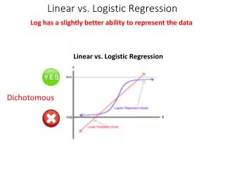
Logistic regression - prediction • Translation from ηi to pi • log{pi/(1- pi)}= β0 + β1xi1 + … + βpxip • Then = logistic function of ηi • Graph of pi versus ηi has a sigmoid shape
GLMs - Inference • The negative inverse Hessian matrix of the log likelihood function characterizes Var( ) (adjunct) • SE( ) obtained as square root of the jth diagonal entry • Typically, substituting for β • “Wald” inference applies the paradigm from Lecture 2 • Z = is asympotically ~ N(0,1) under H0: βj=β0j • Z provides a test statistic for H0: βj=β0j versus HA: βj≠β0j • ± z(1-α/2) SE{ } =(L,U) is a (1-α)x100% CI for βj • {exp(L),exp(U)} is a (1-α)x100% CI for exp(βj)
GLMs: “Global” Inference • Analog: F-testing in linear regression • The only difference: log likelihoods replace SS • Hypothesis to be tested is H0: βj1=...=βjk = 0 • Fit model excluding xj1,...,xjpj: Save -2 log likelihood = Ls • Fit “full” (or larger) model adding xj1,...,xjpj to smaller model. Save -2 log likelihood = LL • Test statistic S = Ls - LL • Distribution under null hypothesis: χ2pj • Define rejection region based on this distribution • Compute S • Reject or not as S is in rejection region or not
GLMs: “Global” Inference • Many programs refer to “deviance” rather than -2 log likelihood • This quantity equals the difference in -2 log likelihoods between ones fitted model and a “saturated model” • Deviance measures “fit” • Differences in deviances can be substituted for differences in -2 log likelihood in the method given on the previous page • Likelihood ratio tests have appealing optimality properties
Outline: A few more topics • Model checking: Residuals, influence points • ML can be written as an iteratively reweighted least squares algorithm • Predictive accuracy • Framework generalizes easily
Main Points • Generalized linear modeling provides a flexible regression framework for a variety of response types • Continuous, categorical measurement scales • Probability distributions tailored to the outcome • Systematic model to accommodate • Measurement range, interpretation • Logistic regression • Binary responses (yes, no) • Bernoulli / binomial distribution • Regression coefficients as log odds ratios for association between predictors and outcomes
Main Points • Generalized linear modeling accommodates description, inference, adjustment with the same flexibility as linear modeling • Inference • “Wald”- statistical tests and confidence intervals via parameter estimator standardization • “Likelihood ratio” / “global” – via comparison of log likelihoods from nested models