Download
1 / 61
610 likes | 733 Views
This study explores the application of Petri Nets in reverse-engineering the business cycle, leveraging microeconomic principles and aggregate data. It critiques traditional DSGE models and considers agent-based modeling as a viable alternative. By analyzing the U.S. economy's input-output tables from 1998 to 2010, the research identifies causal relationships between economic agents' actions and the resulting aggregate outcomes. Key findings include the discovery of complex eigenvalues and their implications for understanding business cycle dynamics over time, particularly post-2007.

E N D
Reverse-Engineering the Business Cycle with Petri Nets Johnnie B. Linn III Concord University Athens, WV
Special Thanks for • Online input-output tables for the U.S. economy, 1998-2010. • U.S. Bureau of Economic Analysis, Department of Commerce, http://www.bea.gov. • Online eigenvalue/eigenvector calculator for a 32 x 32 matrix. • Bluebit Software, http://www.bluebit.gr.
The Problem • “I do not think that the currently popular DSGE models pass the smell test.” • Robert Solow Professor Emeritus, MIT • Prepared Statement, House Committee on Science and Technology Subcommittee on Investigations and Oversight. 1 • So what is DSGE?
Dynamic Stochastic General Equilibrium (DSGE) • Macroeconomic models founded on microeconomic principles.2 • But DSGE failed to foresee the financial crisis. Could agent-based modeling do better? • The Economist, Jul 22nd 2010
Agent-Based Modeling • “[C]omputational models for simulating the actions and interactions of autonomous agents (both individual or collective entities such as organizations or groups) with a view to assessing their effects on the system as a whole.”3
So Where am I Going with This? • The aggregate data we have are the products of agents. Can we find all possible sets of actions of agents that could have produced our results? • Then we can link each set of agents and their actions with a particular set of behavioral assumptions.
Petri Nets • Bipartite Directed Graphs • Used to Model Interconnected Causal Systems
Here, Causal Relationships of Quantities Disposable Income Consumption
Key Assumption • All transitions are enabled, and can be fired in any order. • Makes internal cycles possible. • Models independent actions by agents.
The Business Cycle, Starting Model Value Added Gross Domestic Product
Creation/Destruction Cycle Destructive Processes Gross Domestic Product/ Value Added Intermediate Commodities Creative Processes
Adjacency Matrix for the Creation/Destruction Cycle Int. GDP/VA Total • Creation Process is derived from the transpose of the use table. • Destruction Process is derived from the untransposed use table.
Hard-Wiring the Technical Transformation Processes Int. GDP/VA Total • A token is denominated in dollars. • Arc values can be scaled to best fit the eigenvalue/eigenvector calculating algorithm.
Reverse-Engineering the Cycle • Each firing delivers at least one new token to the cumulative marking. It will be used to fill the element of U that represents that firing. • Working backwards…
where Ct is a vector of constants that ensure that no other elements of U are changed. Continuing.. … So
but so
or • In a cyclical process, U is a set of initial processes C that have replicated themselves.
So let then
The matrix BA’ is a linear transformation of the vector U with eigenvalues (1-νi). Eigenvalues are normally expressed as λ , so we have where λ=1-ν
If the Arcs are Hard-Wired to Data: • The number of tokens accounted for by each element of C will vary according to its process’ contribution to volume. • Likewise the magnitudes of the elements of U will vary according to their processes’ contributions to volume. • The components of U remain orthogonal.
The Data • NIPA Use Tables, 1998-2010 • Two sets • Before redefinitions • After redefinitions • Sector Level
The Computations • 15 creative processes produce 15 commodities plus scrap and noncomparable imports. • 17 destructive processes reduce 15 commodities plus scrap and noncomparable imports to intermediate or final uses. • Scrap and noncomparable imports do not have final uses.
The Computations (2) • There are 32 processes for 18 quantities, so 14 processes are redundant. • (λ I – BA’) is a 32 x 32 matrix. • The matrix has 32 eigenvalues and 32 corresponding eigenvectors. • We seek complex eigenvalues.
Summary of Results • Complex eigenvalues were found. • Average annual angle of rotation (alibi) about 24 degrees. • Corresponds to cycle length of 15 years. • Velocity of rotation increased significantly after 2007. • Phase angles between creation process and corresponding destruction process for each commodity appear to have significance.
What the Algorithm Did • Algorithm had 14 degrees of freedom. • Aligned the phase angles of all 15 creative processes. • Also, rotated each eigenvector to guarantee one process to have a phase angle of zero degrees, or sometimes 180 degrees. • Not always the same process selected.
Agriculture, forestry, fishing, and hunting Before Redefinitions After Redefinitions
Mining Before Redefinitions After Redefinitions
Utilities Before Redefinitions After Redefinitions
Construction Before Redefinitions After Redefinitions
Manufacturing Before Redefinitions After Redefinitions
Wholesale Trade Before Redefinitions After Redefinitions
Retail Trade Before Redefinitions After Redefinitions
Transportation and Warehousing Before Redefinitions After Redefinitions
Information Before Redefinitions After Redefinitions
Finance, insurance, real estate, rental, and leasing Before Redefinitions After Redefinitions
Professional and business services Before Redefinitions After Redefinitions