Activities in Non-Ideal Solutions
210 likes | 509 Views
Activities in Non-Ideal Solutions. Chapter 4 Lecture 10. We will cover Chapter 4 only through section 4.6 (page 144). You will not be responsible for the remaining material in the chapter. Power of Solutions.

Activities in Non-Ideal Solutions
E N D
Presentation Transcript
Activities in Non-Ideal Solutions Chapter 4 Lecture 10
We will cover Chapter 4 only through section 4.6 (page 144). You will not be responsible for the remaining material in the chapter.
Power of Solutions • Our thermodynamics would be so much simpler if all solutions behaved ideally! Even simpler if there were no solutions at all! • But, once we learn how to handle them, we’ll see that we can use solution behavior to do some real geochemistry and learn things about the Earth. • Because the distribution of Mg and Fe between olivine and a magma depends on temperature, we can use the observed distribution to determine magma temperatures. • We can predict the temperature at which K- and Na-feldspar will exsolve and use this to determine metamorphic temperatures. • We can actually predict the plagioclase-spinel peridotite phase transition • We can determine equilibration temperatures of garnet peridotites.
In This Chapter • We’ll learn how to handle non-ideal solutions • Learn how to construct phase diagrams from thermodynamic data • Learn how thermodynamics is used for geothermometry and geobarometry • See how thermodynamics can be used to predict the sequence of minerals precipitating from magma.
Non-Ideality • We found a useful approach to non-ideality in electrolyte solutions (Debye-Hückel), but there are many other kinds of non-ideal solutions, including solids, liquid silicates, etc. • Some substances undergo spontaneous exsolution (oil and water; K- and Na-feldspar; clino- and ortho-pyroxene; silicate and sulfide magmas). When that happens, we know the solution is quite non-ideal (ideal solutions should always be more stable than corresponding physical mixtures).
Margules Equations • When you need to fit an empirical function to an observation and don’t fully understand the underlying phenomena, a power series is a good approach because it of its versatility. • So, for example, we can express the excess volume of a solution (e.g., alcohol and water) as: • where X2is the mole fraction of component 2 and A, B, C, … are constants, Margules parameters, to be determined empirically (e.g., by curve fitting).
Symmetric Solutions • Let’s first look at some simple cases. One such case would be where we need only the first and second order terms. • The excess volume (and other excesses) should be entirely functions of mole fraction, so for a binary solution where X1 = 1 - X2, A= 0 and our equation should reduce to: • The simplest such case would be symmetric about the midpoint X1 = X2. • In that case, • Substituting X1= 1 – X2, we find that B = -C
Interaction Parameters • Let WV = B • W is known as an interaction parameter (volume interaction parameter in this case) because non-ideal behavior results from interactions between dissimilar species. • The interaction parameter is a function of T, P, and the nature of the solution, but not of X. • We can define similar interaction parameters for free energy, enthalpy, and entropy.
Regular Solutions • Since ∆G = ∆H-T∆S • The free energy interaction parameter is: WG =WH – TWS • Regular solutions are the special case where WS = 0 and therefore WG =WH and WG is independent of T. • what does this imply about ∆Sexcess?
Interaction Parameters and Activity Coefficients • For a binary symmetric solution, λ1 must equal λ2 at X1 = X2. • From this we can derive: • For X2 ≈ 1 (very dilute solution of X1), then • and WG = RTln h • What happens when X1 ≈ 1?
Asymmetric Solutions • More complex situation where expansion carried out to third order. • Excess free energy given by: • Activity coefficient: Calculated Free Energy at 600˚C in the Orthoclase-Albite System as a function of Albite mole fraction.
Albite-Orthoclase Free Energy at various T A 3-D version
G-bar–X and Exsolution • We can use G-bar–X diagrams to predict when exsolution will occur. • Our rule is the stable configuration is the one with the lowest free energy. • A solution is stable so long as its free energy is lower than that of a physical mixture. • Gets tricky because the phases in the mixture can be solutions themselves.
Inflection Points • At 800˚C, ∆Greal defines a continuously concave upward path, while at lower temperatures, such as 600˚C (Figure 4.1), inflections occur and there is a region where ∆Greal is concave downward. All this suggests we can use calculus to predict exsolution. • Inflection points occur when curves go from convex to concave (and visa versa). • What property does a function have at these points? • Second derivative is 0. Albite-Orthoclase
Inflection Points • Second derivative is: • First term on r.h.s. is always positive (concave up). • Inflection will occur when
Spinodal Actual solubility gap can be less than predicted because an increase is free energy is required to begin the exsolution process.
Phase Diagrams • Phase diagrams illustrate stability of phases or assemblages of phases as a function of two or more thermodynamic variables (such as P, T, X, V). • Lines mark boundaries where one assemblage reacts to form the other (∆Gr=0).
Thermodynamics of Melting • Melting occurs when free energy of melting, ∆Gm, is 0 (and only when it is 0). • This occurs when: ∆Gm = ∆Hm –T∆Sm • Hence: • Assuming ∆S and ∆H are independent of T: • where Ti,m is the freezing point of pure i, Tis the freezing point of the solution, and the activity is the activity of i in the liquid phase. T-X phase diagram for the system anorthite-diopside.
Computing an Approximate Phase Diagram We assume the liquid is an ideal solution (ai = Xi) and compute over the range of Xi