Principles and Practice of Application Performance Measurement and Analysis on Parallel Systems

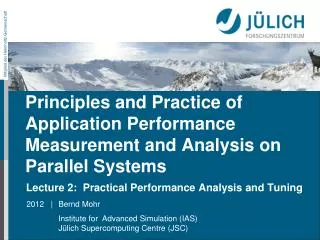
Principles and Practice of Application PerformanceMeasurement and Analysis on Parallel Systems Lecture 1: Terminology and Methodology 2012 | Bernd Mohr Institute for Advanced Simulation (IAS) Jülich Supercomputing Centre (JSC)

Performance Tuning: an Old Problem! [Intentionally left blank]

Performance Tuning: an Even Older Problem!! “The most constant difficulty in contriving the engine has arisen from the desire to reduce the time in which the calculations were executed to the shortest which is possible.” Charles Babbage 1791 - 1871

Motivation • High complexity in parallel and distributed systems • Four layers • Application • Algorithm, data structures • Parallel programming interface / Middle ware • Compiler, parallel libraries, communication, synchronization • Operating system • Process and memory management, IO • Hardware • CPU, memory, network • Mapping/interaction between different layers

Performance Properties of Parallel Programs  Choose right algorithm, use optimizing compiler  Tough! Not many tools yet, hope compiler gets it right  Not given enough attention  More or less understood, tool support • Factors which influence performance of parallel programs • “Sequential” factors • Computation • Cache and memory • Input / output • “Parallel” factors • Communication (Message passing) • Threading • Synchronization

Transformation of the results into arepresentation that can be easilyunderstood by a human user • Collection of data relevant toperformance analysis • Elimination of performance problems • Calculation of metrics, identification of performance problems Measurement Analysis Presentation Optimization Performance Measurement Cycle Instrumentation • Insertion of extra code (probes, hooks)into application

Metrics • Instrumentation techniques • Source code instrumentation • Binary instrumentation • Instrumentation of parallel programs • MPI • OpenMP • Measurement techniques • Profiling • Tracing

Metrics of Performance • What can be measured? • A count of how many times an event occurs • E.g., Number of input / output requests • The duration of some time interval • E.g., duration of these requests • The size of some parameter • Number of bytes transmitted or stored • Derived metrics • E.g., rates / throughput • Needed for normalization

Example Metrics • Clock rate • MIPS • Millions of instructions executed per second • FLOPS • Floating-point operations per second • Benchmarks • Standard test program(s) • Standardized methodology • E.g., SPEC, Linpack • QUIPS / HINT [Gustafson and Snell, 95] • Quality improvements per second • Quality of solution instead of effort to reach it • Execution time “math” Operations? HW Operations? HW Instructions? 32-/64-bit? …

Execution Time • Wall-clock time • Includes waiting time: IO, memory, other system activities • In time-sharing environments also time consumed by other applications • CPU time • Time spent by the CPU to execute the program • Execution time on behalf of the program • Does not include time the program was context-switched out • Problem: does not include inherent waiting time (e.g., IO) • Problem: portability? What is user, what is system time? • Problem: execution time is non-deterministic • Use mean or minimum of several runs

Load Imbalance Metrics Computation Imbalance Time = Max Time – Avg time Synchronization Imbalance Time = Avg Time – Min time • Synchronization Imbalance Time • Provides an estimation to the user of how much time in the overall program would be saved if the corresponding section of the code had a perfect balance • Represents an upper bound on the “potential saving” • Imbalance Time • Metric time to identify code regions that need optimization • Two variations: • Computation Imbalance Time I-11

Imbalance time N Imbalance% = 100 X X Max Time N - 1 Load Imbalance Metrics I-12 • Imbalance % • Provide an idea of the “badness” of the imbalance • Corresponds to the % of the time that the rest of the team, excluding the slowest PE is not engaged in useful work on the given function • “Percentage of resources available for parallelism” that is wasted

Speedup and Efficiency • For a given problem A, let • SerTime(n) = Time of the best serial algorithm to solve A for input of size n • ParTime(n,p) = Time of the parallel algorithm + architecture to solve A for input size n, using p processors • Note that SerTime(n) ≤ ParTime(n,1) • Then • Speedup(p) = SerTime(n) / ParTime(n,p) • Work(p) = p • ParTime(n,p) • Efficiency(p) = SerTime(n) / [p • ParTime(n,p)]

Speedup and Efficiency II • In general, expect • 0 ≤ Speedup(p) ≤ p • Serial work ≤ Parallel work < ∞ • 0 ≤ Efficiency ≤ 1 • Linear speedup: if there is a constant c > 0 so that speedup is at least c • p. Many use this term to mean c = 1. • Perfect or ideal speedup: speedup(p) = p • Superlinear speedup: speedup(p) > p (effiency > 1) • Typical reason: Parallel computer has p times more memory (cache), so higher fraction of program data fits in memory instead of disk (cache instead of memory) • Parallel version is solving slightly different, easier problem or provides slightly different answer

Amdahl’s Law • Amdahl [1967] noted: • Given a program, let f be fraction of time spent on operations that must be performed serially (unparallelizable work). Then for p processors: 1 Speedup(p) ≤ f + (1 – f)/p • Thus no matter how many processors are used Speedup(p) ≤ 1/f • Unfortunately, typical f is 5 – 20%

Maximal Possible Speedup / Efficiency f=0.001 f=0.01 f=0.1

Amdahl’s Law II • Amdahl was an optimist • Parallelization might require extra work, typically • Communication • Synchronization • Load balancing • Amdahl convinced many people that general-purpose parallel computing was not viable • Amdahl was an pessimist • Fortunately, we can break the law! • Find better (parallel) algorithms with much smaller values of f • Superlinear speedup because of more data fits cache/memory • Scaling: time spent in serial portion is often a decreasing fraction of the total time as problem size increase I-17

Scaling • Sometimes the serial portion • is a fixed amount of time independent of problem size • or grows with problem size but slower than total time • Thus can often exploit large parallel machines by scaling the problem size with the number of processes • Scaling approaches used for speedup reporting/measurements: • Fixed problem size (strong scaling) • Fixed problem size per processor (weak scaling) • Fixed time, find largest problem solvable [Gustafson 1988]Commonly used in evaluating databases (transactions/s) • Fixed efficiency: find smallest problem to achieve it(isoefficiency analysis)

... v09,S [a30,1],m00 a30 -26612:abcd v12,S [a31,1],m00 a30 a12+a30 a31 -26616:abcd v10,S [a30,1],m00 a16 -22516:abcd a31 a12+a31 a30 a15+a16 v14,S [a31,1],m00 a16 -32764:abcd v11,S v10-v14,m00 ... C = A + B (c1, c2) = (a1, a2) 6 (b1, b2) a1=1& a2=1e c1bb1& c2bb2 b1=1& b2=1e c1ba1& c2ba2 for i = 1 : 2, ai=? e ci b bi bi=? e ci b ai ai= bi e ci b ai otherwise, error Performance Tools Challenge • User’s mental model of the programdoes not match the executed version • Performance tools must be able to revert this semantic gap

Semantic Gap • Instrumentation levels • Source code • Library • Runtime system • Object code • Operating system • Runtime image • Virtual machine • Problem • Every level provides different information • Often instrumentation on multiple levels required • Challenge • Mapping performance data onto application-level abstraction

Instrumentation Techniques • Static instrumentation • Program is instrumented prior to execution • Dynamic instrumentation • Program is instrumented at runtime • Code is inserted • Manually • Automatically • By preprocessor / source-to-source translation tool • By compiler • By linking against pre-instrumented library or runtime system • By binary-rewrite / dynamic instrumentation tool  e.g., “printf”  manual static source-code instrumentation

int func(...) { double d; trace_enter(); return (foo()*bar()); trace_exit(); } Source Code Instrumentation (I) • For large complex applications, manual instrumentation is too tediousand error-prone  Tool support needed • Automatic performance Instrumentation typically requires full source code parsers, e.g., • Fortran, C: find 1st executable line and all exit points • C: executable code inside return statements int func(...) { double d; return (foo()*bar()); } int func(...) { double d; trace_enter(); trace_exit(); return (foo()*bar()); } int func(...) { double d; trace_enter(); { int t1_ = (foo()*bar()); trace_exit(); return t1_; } }

Source Code Instrumentation (II) • Example C++ issues: • Template instrumentation? • Executing code before main • C++ instrumentation trick • Define instrumentation object • Declare instrumentation object as 1st statement in every function and method to be instrumented • Function overloading • Operator overloading class Tracer { public: Tracer(…) { trace_enter(); } ~Tracer() { trace_exit(); } }; int func(...) { Tracer trc_1; double d; return (foo()*bar()); }

TAU Source Code Instrumentor • Part of the TAU performance framework • Supports • f77, f90 • C, and C++ • Inserts calls to the TAU monitoring API • Based on the Program Database Toolkit • http://tau.uoregon.edu/

Program Database Toolkit • Based on commercial parsers • C, C++: Edison Design Group (EDG) • Full ISO 1998 C++ and ISO 1999 C Support • Fortran 77, Fortran90: Mutek, [Cleanscape] • Program Database Utilities and ConversionTools APplication Environment (DUCTAPE) • Object-oriented Access to Static Information • Classes, Modules, Routines, Types, Templates, Files, Macros, Namespaces, Comments/Pragmas, Statements (C/C++ only) • http://www.cs.uoregon.edu/research/pdt/

PDT Architecture and Tools Application / Library C / C++ parser Fortran parser F77/90/95 Program documentation PDBhtml Application component glue IL IL SILOON C / C++ IL analyzer Fortran IL analyzer C++ / F90/95 interoperability CHASM DUCTAPE Program Database Files Automatic source instrumentation TAU_instr

Binary Instrumentation • Static binary rewrite • Instrumentation code is insertedinto the binary before it starts to execute • Creates modified executable • Dynamic binary instrumentation • On-the-fly: Insert, remove, and change instrumentationin the application program while it is running • Most flexible (but most complex) technique • Parallel programs  Coordinated instrumentation of all images needed

Dyninst • Dyninst is a C++ library for machine-independent • process control and manipulation • runtime code generation • and binary patching • University of Wisconsin and University of Maryland • Basis for Paradyn, DPCL, and OpenSpeedShop • Open source • Supports • Power/PowerPC (Linux) • BlueGene/P • http://www.dyninst.org • X86 (Linux, BSD, Windows) • X86_64 (Linux, BSD, Windows)

Comparison of Techniques (I) • Source code instrumentation • Portable • Link back to source code easy • Only way to capture “high-level” user abstractions • Recompilation necessary for (change in) instrumentation • Requires source code to be available • Hard to use for mixed-language applications • Source-to-source translation tool hard to implement for C++ and Fortran90

Comparison of Techniques (II) • Binary code instrumentation • / The other way around compared to source instrumentation • Pre-instrumented library / runtime • Easy to use: only re-linking necessary • Can only record information about library / runtime entities • No single technique is sufficient! • Typically, combinations of techniques needed!

Instrumentation of Parallel Programs • User-level constructs • Modules / components / … • Program phases • Functions • Loops • … • Constructs of the parallel programming models • Message passing • MPI, PVM, … • Threading and synchronization • OpenMP, POSIX, Win32, or Java threads, …

Instrumentation of User Functions • Ideally: instrumentation by compiler or tool • Hidden, unsupported compiler options(GNU, Intel, IBM, NEC, Sun Fortran, PGI, Hitachi, ???) • TAU Source Code Instrumentor • TAU Binary Instrumentor (Dyninst) • TAU Virtual Machine Instrumentor (Java, Python) • Always works: manually • Instrumentation APIs of tools: Scalasca, Vampirtrace, TAU, … • Scalasca’s POMP Directives • More details later … • Main problem: selection of relevant constructs

Wrapper Library MPI Library MPI Library MPI_Send MPI_Send MPI_Send PMPI_Send PMPI_Send MPI_Bcast MPI_Bcast PMPI: The MPI Profiling Interface • Every MPI function has two names: MPI_xxx and PMPI_xxx • This allows selective replacement of MPI routines at link time no re-compilation necessary • Also called: wrapper function library • Used by basically every MPI performance tools • VampirTrace, MPICH MPE, Scalasca EPIK, TAU, … User Program Call MPI_Send Call MPI_Bcast

PMPI Example (C/C++) #include <stdio.h> #include "mpi.h" static int numsend = 0; int MPI_Send(void *buf, int count, MPI_Datatype type, int dest, int tag, MPI_Comm comm) { numsend++; return PMPI_Send(buf, count, type, dest, tag, comm); } int MPI_Finalize() { int me; PMPI_Comm_rank(MPI_COMM_WORLD, &me); printf("%d sent %d messages.\n", me, numsend); return PMPI_Finalize(); }

PMPI Wrapper Development • MPI has many functions! [MPI-1: 130 MPI-2: 320] use wrapper generator (e.g., from MPICH MPE)  needed for Fortran and C/C++ • Message analysis / recording • Location recording  use ranks in MPI_COMM_WORLD? • Data volume #elements * sizeof(type) • No message ID  need complete recording of traffic • Wildcard source and tag  record real values • Collective communication  communicator tracking • Non-blocking, persistent communication  track requests • Non-blocking  record recv at Wait*, Test*, Irecv ? • One-sided communication?

OpenMP Monitoring? • Problem: • OpenMP does not define standard monitoring interface • OpenMP is defined mainly by directives/pragmas • Solution: • POMP: OpenMP Monitoring Interface • Joint Development • Forschungszentrum Jülich • University of Oregon • Presented at EWOMP’01, LACSI’01 and SC’01 “The Journal of Supercomputing”, 23, Aug. 2002.

Example:!$OMP PARALLEL DO POMP Instrumentation context descriptor !$OMP PARALLEL DO clauses...do loop!$OMP END PARALLEL DO !$OMP PARALLEL other-clauses... !$OMP DO schedule-clauses, ordered-clauses,lastprivate-clausesdo loop !$OMP END DO !$OMP END PARALLEL DO NOWAIT!$OMP BARRIER call pomp_parallel_fork(d1)call pomp_parallel_begin(d1)call pomp_parallel_end(d1)call pomp_parallel_join(d1) call pomp_do_enter(d2)call pomp_do_exit(d2) call pomp_barrier_enter(d3)call pomp_barrier_exit(d3)

POMP-like Hooks in Production Compilers • POMP was the base for the OpenMP instrumentation hooks provided in production compilers • Cray Compiling Environment • PGI • IBM XL compilers • These instrumentation hooks are used for performance analysis of OpenMP in production tools • CrayPat • PGProf • Also: New OpenMP ARB sanctioned low-level tool interface • http://www.compunity.org/futures/omp-api.html • Proof-of-concept implementations by Sun and Intel compilers

POMP Instrumentation Tool • OpenMPPragmaAnd Region Instrumentor • Source-to-source translator to insert POMP callsaround OpenMP constructs and API functions • Implemented in C++ • Supports: • Fortran77 und Fortran90, OpenMP 3.0 • C und C++,OpenMP 3.0 • Additional POMP directives for control and region definition • Used by Scalasca, VampirTrace, TAU, and ompP • Preserves source code information (#line line file) • Does not support: Instrumentation of user functions

Current Major OPARI Limitations Fixed in OPARI2 Fixed in OPARI2 • Does not yet support • Varying number of threads in different parallel regions • Nested parallelism • Latest OpenMP 3.0 standard features like tasking • Executed before compiler preprocessor issues with macros, conditional compilation, includes! • Needs special care if building ... • ... more than one application in one directory • ... applications spread over multiple directories

Performance Measurement • Two dimensions • When performance measurement is triggered • External agent (asynchronous) • Sampling • Timer interrupt • Hardware counters overflow • Can measure unmodified executables, very low overhead • Internal agent (synchronous) • Code instrumentation: • Automatic or manual instrumentation • How performance data is recorded • Profile ::= Summation of events over time • run time summarization (functions, call sites, loops, …) • Trace file ::= Sequence of events over time

inclusive duration exclusive duration child duration Measurement • Typical performance data include • Counts • Durations • Communication cost • Synchronization cost • IO accesses • System calls • Hardware events int f1() { int a; a = a + 1; f2(); a = a + 1; return a; }

Critical Issues • Accuracy • Perturbation • Measurement alters program behavior • E.g., memory access pattern • Intrusion overhead • Measurement itself needs time and thus lowers performance • Accuracy of timers, counters • Granularity • How many measurements • How much information / work during each measurement • Tradeoff • Accuracy  expressiveness of data

Measurement Methods: Profiling • Recording of aggregated information • Time • Counts • Calls • Hardware counters • about program and system entities • Functions, call sites, loops, basic blocks, … • Processes, threads • Methods to create a profile • PC sampling (statistical approach) • Interval timer / direct measurement (deterministic approach)

Profiling (2) • Sampling • General statistical measurement technique based on the assumption that a subset of a population being examined is representative for the whole population • Running program is interrupted periodically • Operating system signal or Hardware counter overflow • Interrupt service routine examines return-address stack to find address of instruction being executed when interrupt occurred • Using symbol-table information this address is mapped onto specific subroutine • Requires long-running programs • Interval timing • Time measurement at the beginning andat the end of a code region • Requires instrumentation + high-resolution / low-overhead clock

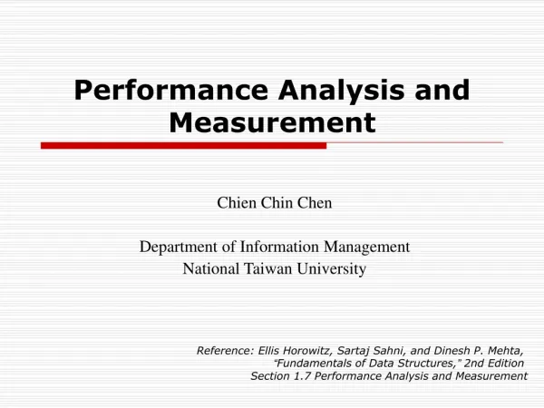
Measurement Methods: Tracing • Recording information about significant points (events) during execution of the program • Enter/leave a code region (function, loop, …) • Send/receive a message ... • Save information in event record • Timestamp, location ID, event type • plus event specific information • Event trace := stream of event records sorted by time • Can be used to reconstruct the dynamic behavior  Abstract execution model on level of defined events

... 2 1 bar foo ... 60 64 58 ... 68 69 62 B A B A A B EXIT SEND RECV ENTER ENTER EXIT 1 2 2 A B 1 Event tracing Local trace A ... ... Process A Global trace 58 60 ENTER ENTER 1 1 void foo() { trc_enter("foo"); ... trc_send(B); send(B, tag, buf); ... trc_exit("foo"); } void foo() { ... send(B, tag, buf); ... } MONITOR 68 62 RECV SEND A B 64 69 EXIT EXIT 1 1 ... ... 1 1 bar foo ... ... Local trace B instrument synchronize(d) Process B merge void bar() { ... recv(A, tag, buf); ... } void bar() { trc_enter("bar"); ... recv(A, tag, buf); trc_recv(A); ... trc_exit("bar"); } unify MONITOR

Principles and Practice of Application Performance Measurement and Analysis on Parallel Systems