
Singular Value Decomposition & Underconstrained Least Squares
E N D
Presentation Transcript
Underconstrained Least Squares • What if you have fewer data points than parameters in your function? • Intuitively, can’t do standard least squares • Recall that solution takes the form ATAx = ATb • When A has more columns than rows,ATA is singular: can’t take its inverse, etc.
Underconstrained Least Squares • More subtle version: more data points than unknowns, but data poorly constrains function • Example: fitting to y=ax2+bx+c
Underconstrained Least Squares • Problem: if problem very close to singular, roundoff error can have a huge effect • Even on “well-determined” values! • Can detect this: • Uncertainty proportional to covariance C = (ATA)-1 • In other words, unstable if ATA has small values • More precisely, care if xT(ATA)x is small for any x • Idea: if part of solution unstable, set answer to 0 • Avoid corrupting good parts of answer
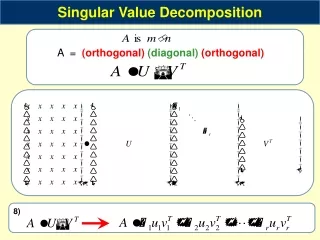
Singular Value Decomposition (SVD) • Handy mathematical technique that has application to many problems • Given any mn matrix A, algorithm to find matrices U, V, and W such that A = UWVT U is mn and orthonormal W is nn and diagonal V is nn and orthonormal
SVD • Treat as black box: code widely availableIn Matlab: [U,W,V]=svd(A,0)
SVD • The wi are called the singular values of A • If A is singular, some of the wiwill be 0 • In general rank(A) = number of nonzero wi • SVD is mostly unique (up to permutation of singular values, or if some wi are equal)
SVD and Inverses • Why is SVD so useful? • Application #1: inverses • A-1=(VT)-1W-1U-1 = VW-1UT • Using fact that inverse = transposefor orthogonal matrices • Since W is diagonal, W-1 also diagonal with reciprocals of entries of W
SVD and Inverses • A-1=(VT)-1W-1U-1 = VW-1UT • This fails when some wi are 0 • It’s supposed to fail – singular matrix • Pseudoinverse: if wi=0, set 1/wi to 0 (!) • “Closest” matrix to inverse • Defined for all (even non-square, singular, etc.) matrices • Equal to (ATA)-1AT if ATA invertible
SVD and Least Squares • Solving Ax=b by least squares • x=pseudoinverse(A) times b • Compute pseudoinverse using SVD • Lets you see if data is singular • Even if not singular, ratio of max to min singular values (condition number) tells you how stable the solution will be • Set 1/wi to 0 if wi is small (even if not exactly 0)
SVD and Eigenvectors • Let A=UWVT, and let xi be ith column of V • Consider ATAxi: • So elements of W are sqrt(eigenvalues) and columns of V are eigenvectors of ATA • What we wanted for robust least squares fitting!
SVD and Matrix Similarity • One common definition for the norm of a matrix is the Frobenius norm: • Frobenius norm can be computed from SVD • So changes to a matrix can be evaluated by looking at changes to singular values
SVD and Matrix Similarity • Suppose you want to find best rank-k approximation to A • Answer: set all but the largest k singular values to zero • Can form compact representation by eliminating columns of U and V corresponding to zeroed wi
* * Second principal component * * First principal component * * * * * * * * * * * * * * * * * * * * Data points SVD and PCA • Principal Components Analysis (PCA): approximating a high-dimensional data setwith a lower-dimensional subspace Original axes
SVD and PCA • Data matrix with points as rows, take SVD • Subtract out mean (“whitening”) • Columns of Vk are principal components • Value of wi gives importance of each component
PCA on Faces: “Eigenfaces” First principal component Averageface Othercomponents For all except average,“gray” = 0,“white” > 0, “black” < 0
Using PCA for Recognition • Store each person as coefficients of projection onto first few principal components • Compute projections of target image, compare to database (“nearest neighbor classifier”)
Total Least Squares • One final least squares application • Fitting a line: vertical vs. perpendicular error
Total Least Squares • Distance from point to line:where n is normal vector to line, a is a constant • Minimize:
Total Least Squares • First, let’s pretend we know n, solve for a • Then
Total Least Squares • So, let’s defineand minimize
Total Least Squares • Write as linear system • Have An=0 • Problem: lots of n are solutions, including n=0 • Standard least squares will, in fact, return n=0
Constrained Optimization • Solution: constrain n to be unit length • So, try to minimize |An|2 subject to |n|2=1 • Expand in eigenvectors ei of ATA:where the i are eigenvalues of ATA
Constrained Optimization • To minimize subject toset min = 1, all other i = 0 • That is, n is eigenvector of ATA withthe smallest corresponding eigenvalue