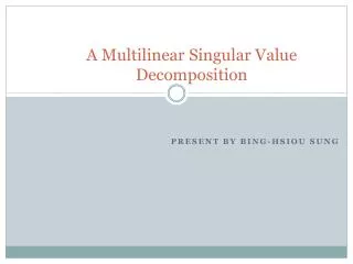
Singular Value Decomposition SVD
Singular Value Decomposition SVD. Week 9. SVD - Detailed outline. Linear Algebra review Motivation Definition - properties Interpretation Complexity Case studies Additional properties. Vector. Vector length Vector addition. Vector (cont ’ d). Scalar multiplication

Singular Value Decomposition SVD
E N D
Presentation Transcript
SVD - Detailed outline • Linear Algebra review • Motivation • Definition - properties • Interpretation • Complexity • Case studies • Additional properties
Vector • Vector length • Vector addition
Vector (cont’d) • Scalar multiplication • Multiplying a scalar (real number) times a vector means multiplying every component by that real number to yield a new vector. • Inner product (dot product)
Orthogonality • Two vector are orthogonal to each other if their inner product equals zero. • In two-dimensional space, this is equivalent to saying that the vectors are perpendicular, or that the only angle between them is a 90◦ angle.
Normal Vector • A normal vector (or unit vector) is a vector of length 1. • Any vector with an initial length > 0 can be normalized by dividing each component in it by the vector’s length.
Orthonormal Vector • Vectors of unit length that are orthogonal to each other are said to be orthonormal.
Gram-Schmidt Orthonormalization Process • It is a method for converting a set of vectors into a set of orthonormal vectors. • It basically begins by normalizing the first vector under consideration and iteratively rewriting the remaining vectors in terms of themselves minus a multiplication of the already normalized vectors. • Normalize the first vector to • For the second vector • Normalize it to get
Matrix • Square matrix • Matrix transpose • Matrix multiplication • Identity matrix • Orthogonal matrix • Diagonal matrix
Eigenvector / Eigenvalue • An eigenvector is a nonzero vector that satisfies the equation where A is a square matrix, λ is a scalar, and is the eigenvector. λ is called an eigenvalue.
SVD - Detailed outline • Linear Algebra review • Motivation • Definition - properties • Interpretation • Complexity • Distributed SVD on Mahout
SVD - Motivation • problem #1: text - LSI: find ‘concepts’ • problem #2: compression / dim. reduction
SVD - Motivation • problem #1: text - LSI: find ‘concepts’
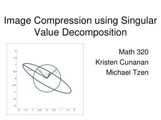
SVD - Motivation • problem #2: compress / reduce dimensionality
Problem - specs • ~10**6 rows; ~10**3 columns; no updates; • random access to any cell(s) ; small error: OK
SVD - Detailed outline • Linear Algebra review • Motivation • Definition - properties • Interpretation • Complexity • Distributed SVD on Mahout
SVD - Definition (reminder: matrix multiplication) x = 3 x 2 2 x 1
SVD - Definition (reminder: matrix multiplication x = 3 x 2 2 x 1 3 x 1
SVD - Definition (reminder: matrix multiplication x = 3 x 2 2 x 1 3 x 1
SVD - Definition (reminder: matrix multiplication x = 3 x 2 2 x 1 3 x 1
SVD - Definition (reminder: matrix multiplication x =
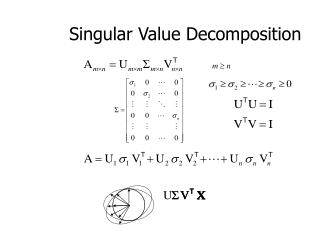
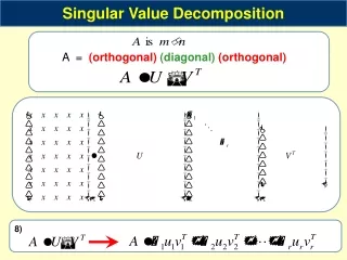
SVD - Definition A[n x m] = U[n x r]L [ r x r] (V[m x r])T • A: n x m matrix (eg., n documents, m terms) • U: n x r matrix (n documents, r concepts) • L: r x r diagonal matrix (strength of each ‘concept’) (r : rank of the matrix) • V: m x r matrix (m terms, r concepts)
SVD - Definition • A = ULVT - example:
SVD - Properties THEOREM [Press+92]:always possible to decomposematrix A into A = ULVT , where • U,L,V: unique (*) • U, V: column orthonormal (ie., columns are unit vectors, orthogonal to each other) • UTU = I; VTV = I (I: identity matrix) • L: eigenvalues are positive, and sorted in decreasing order
SVD - Example • A = ULVT - example: retrieval inf. lung brain data CS x x = MD
SVD - Example • A = ULVT - example: retrieval CS-concept inf. lung MD-concept brain data CS x x = MD
SVD - Example • A = ULVT - example: doc-to-concept similarity matrix retrieval CS-concept inf. lung MD-concept brain data CS x x = MD
SVD - Example • A = ULVT - example: retrieval ‘strength’ of CS-concept inf. lung brain data CS x x = MD
SVD - Example • A = ULVT - example: term-to-concept similarity matrix retrieval inf. lung brain data CS-concept CS x x = MD
SVD - Example • A = ULVT - example: term-to-concept similarity matrix retrieval inf. lung brain data CS-concept CS x x = MD
SVD - Detailed outline • Linear Algebra review • Motivation • Definition - properties • Interpretation • Complexity • Distributed SVD on Mahout
SVD - Interpretation #1 ‘documents’, ‘terms’ and ‘concepts’: • U: document-to-concept similarity matrix • V: term-to-concept sim. matrix • L: its diagonal elements: ‘strength’ of each concept
SVD - Interpretation #2 • best axis to project on: (‘best’ = min sum of squares of projection errors)
minimum RMS error SVD - interpretation #2 SVD: gives best axis to project v1
x x = v1 SVD - Interpretation #2 • A = ULVT - example:
SVD - Interpretation #2 • A = ULVT - example: variance (‘spread’) on the v1 axis x x =
SVD - Interpretation #2 • A = ULVT - example: • UL gives the coordinates of the points in the projection axis x x =
x x = SVD - Interpretation #2 • More details • Q: how exactly is dim. reduction done?
SVD - Interpretation #2 • More details • Q: how exactly is dim. reduction done? • A: set the smallest eigenvalues to zero: x x =
SVD - Interpretation #2 x x ~
SVD - Interpretation #2 x x ~
SVD - Interpretation #2 x x ~
SVD - Interpretation #2 Exactly equivalent: ‘spectral decomposition’ of the matrix: x x =
SVD - Interpretation #2 Exactly equivalent: ‘spectral decomposition’ of the matrix: l1 x x = u1 u2 l2 v1 v2
l1 l2 u1 u2 vT1 vT2 SVD - Interpretation #2 Exactly equivalent: ‘spectral decomposition’ of the matrix: m = + +... n