Download
1 / 53
530 likes | 615 Views
Interpreting Seismic Observables Geoff Abers, Greg Hirth. Velocities: compositional effects vs P,T Attenuation at high P, T Anisotropy ( Hirth ). Upload from bSpace -> Seismic_Properties : Hacker&AbersMacro08Dec2010.xls & various papers. A random tomographic image.

E N D
Interpreting Seismic ObservablesGeoff Abers, Greg Hirth Velocities: compositional effects vs P,T Attenuation at high P, T Anisotropy (Hirth) Upload from bSpace -> Seismic_Properties: Hacker&AbersMacro08Dec2010.xls & various papers
A random tomographic image Crustal tomography: Woodlark Rift, Papua New Guinea - Transition from continental to oceanic crust (Ferris et al., 2006 GJI)
Arc crust velocities Arc Vp along-strike Aleutians Vs. SiO2 in arc lavas [Shillington et al., 2004] Arc lower crust predictions [Behn & Kelemen, 2006]
Velocity variations within subducting slab dlnVs = 10-15% E W km from coast dlnVs = 2-4% CAFE Transect, Washington Cascades (Abers et al., Geology, 2009) Green: relocated, same velocities. yellow: catalog hypocenters
Unusual low Vp/Vs in wedge * PREM: Vp = 8.04 km/s, Vp/Vs = 1.80 Vp/Vs = 1.65-1.70 Vp/Vs = 1.8-1.9 Alaska (Rossi et al. 2006) Andes 31°S (Wagner et al. 2004) “Normal” N Honshu Zhang et al. (Geology 2004) Strange: no volcanics
%Vp/VpHARZ 100 92 %Vp ~ 99-103 % (eclogite/peridotite) %Vp ~ 85-95 % (hydrated/peridotite) 87 95 84 81 Velocities & H2O in metabasalts • Crust Hydrated at: • low P, or • low T eclogite blueschist amphibolite gr-sch (Hacker et al., 2003a JGR; Hacker & Abers, 2004 Gcubed)
What else affects velocities? (b) temperature (c) fluids Pore fluids k melts Temperature H2O = bulk modulus = shear modulus Takei (2002) poroelastic theory aspect ratio 0.1-0.5 Faul & Jackson (2005) anelasticity + anharmonicity
Two Approaches • (1) Direct measurement of rock velocities
V vs. composition… Crustal rock variations Brocher, 2005 Arc lower crust Behn & Kelemen 2006
Second Approach Disaggregate rock into mineral modal abundances • (2) Measure/calculate mineral properties, and aggregate For each mineral, look up K, G, V, … at STP & derivatives Peridotites: Lee, 2003 Extrapolate K(P,T), G(P,T), … Aggregate to crystal mixture Calculate Vp, Vs Eclogite: Abalos et al., GSABull 2011
Whole-rock vs. calculated velocities (Oceanic gabbros, from Carlson et al., Gcubed 2009)
Measured vs predicted Vp • Oceanic gabbros (data) • Thick line: predictions • What is going on? Behn & Kelemen, 2003 Gcubed
Calculating seismic velocities from mineralogy, P,T(Hacker et al., 2003, JGR; Hacker & Abers 2004, Gcubed) elastic parameters Thermodynamic parameters for 55 end-member minerals - 3rd order finite strain EOS - aggregated by solid mixing thy. Track V, , H2O, major elem., T,P minerals
Compiled Parameters • ro=r(P=0 GPa,T=25 C) = density • KT0 = isothermal bulk modulus (STP) • G0= shear modulus (STP) • a0; da/dTor similar = coef. Thermal expansion • K’ = dKT/dP = pressure derivative • G = dlnG/dlnr= T derivative (G(T)) • G’ = dG/dP = pressure derivative • gth= 1st (thermal) Grüneisen parameter • dT = 2nd (adiabatic) Grüneisen parameter (K(T))
Elastic Moduli vs. P, T • Computational Strategy: • First increase T • thermal expansion… • Second increase P • 3rd order finite strain EoS Integrate in P STP Integrate in T From Hacker et al. 2003a
Aggregating & Velocities • Mixture theories, simple: Voight-Reuss-Hill • average K, 1/K, both • Complex Hashin-Shtrikman Mixtures • sorted/weighted averages Finally, turn elastic parameters to seismic velocities using the usual…
Usage notes “Raw” data table: elastic parameters & derivatives Intermediate calculation table Work table: Enter compositions, P,T here Mineralinformation & stored compositions “database” includes references & notes on source of values
Usage notes: rocks mins modes Petrology for people who don’t know the secret codes Compositions from Hacker et al. 2003 Metagabbros Metaperidotites
Usage Notes: you manipulate “rocks” sheet Enter compositions here… (adds to 100%) … and P,T here… (optional: d, f for anelastic correction) (primary output) …then click to run More info below
The mineral database – how good? Dry, major mantle minerals: OK Hydrous, and/or highly anisotropic..??? Shear Modulus (& derivatives)???
Inside the macro… V r a0 KT K’ G G’ g dth Yellow: extrapolated, calculated from related parameters, or otherwise indirect Big problems w/ shear modulus
A couple of Apps… use “Perple_X” to calculate phases, HAMacro to calculate velocities Hydrated metabasalts (after Hacker, 2008; Hacker and Abers, 2004)
Predict T(P) from model (Abers et al., 2006, EPSL) & Facies from petrology (Hacker et al., 2003)
Predictions from thermal/petrologic model H2O Vs 2D model predictions
Serpentinization effect on Vp Are downgoing plates serpentinized? (Nicaragua forearc) [Hyndman and Peacock, 2003]
Result: low Vp/Vs in “deeper” wedge Where slab is deep: Vp/Vs = 1.64-1.69 (consistent w/ tomography)
The Andes [Wagner et al., 2004, JGR] 31.1°S Flat Slab Vp/Vs < 1.68-1.72 32.6°S
Vp/Vs and composition: need quartz Andes AK wedge
What is seismic attenuation? Q = DE/E - loss of energy per cycle DE T 1/f Amplitude ~ exp(-pftT/Q)
What Causes Attenuation? Upper Crust:cracks, pores Normal Mantle:thermally activated dissipation Cold Slabs:?? (scattering may dominate if 1/Qintrinsic is low)
Seismic Attenuation (1/Q) at high T • At High T, Q Has: • strong T sensitivity • some to H2O, grain size, melt • weak compositional sensitivity • shear, not bulk 1/Q d=1 mm 10 mm Faul & Jackson (2005), adjusted to 2.5 GPa
High-Temperature Background (HTB) Simple model (Jackson et al. 2002) grain size activation energy period temperature • = 0.2-0.3 (frequency dep.) • m = a (grain size dep.)
Attenuating Signals RCK DH1 updip DH1 = 0.92° RCK = 0.91° wedge 2 s P waves depth 126 km (Stachnik et al., 2004, JGR)
Forearc Path Wedge Path S waves, slab event, D ~ 100 km Q Measurements Q and amplitude u(f): u(f) = U0Asource(f) e-pfT/Q Fit P, S spectra: T/Q, M0, fc 0.5 – (10-20) Hz
Path-averaged Qs Invert these tomographically assumes Q(f) from laboratory predictions
Test of Q theory: Ratio of Bulk / Shear attenuation high 1/Qs high 1/Qk Alaska cross-section (Stachnik et al., 2004)
Test of HTB: Frequency Dependence Q = Q0fa Lab: Faul & Jackson 2005 Observations from Alaska
Forearcs: cold; subarc mantle: hot Heat flow in northern Cascadia: step 20-30 km from arc (Wada and Wang, 2009; after Wang et al. 2005; Currie et al., 2004)
hi Q lo Q Results from Alaska (BEAAR): 1/QS In wedge core: QS ~ 100-140 @ 1 Hz 1200-1400°C (dry) (Stachnik et al., 2004 JGR)
Attenuation in Central America (TUCAN) (Rychert et al., 2008 G-Cubed)
Attenuation vs Velocity: Physical Dispersion “Attenuation” without causality No attenuation Attenuation + Causality = Delay in high-frequency energy
Attenuation vs Velocity: Physical Dispersion • This means: • Band-limited measurements of travel time are late • Band-limited measures give slower apparent velocities • As T increases, both V and Q decrease No attenuation Attenuation + Causality
Physical Dispersion: Faul/Jackson approx. K anharmonic G anharmonic + anelastic
Physical Dispersion: Karato approx. Karato, 1993 GRL
Net effect: interpreting DT from DVs Faul & Jackson, 2005 EPSL
Deep under the hood: adiabatic vs. isothermal Important distinction between adiabatic (const. S) and isothermal (const. T) processes Labs & petrologists usually measure this Seismic waves see this (not the same!) Useful: Bina & Helffrich, 1992 Ann. Rev.; Hacker and Abers, 2004 GCubed