Download
1 / 74
750 likes | 784 Views
Explore market structure characteristics and competition dynamics in the livestock industry, including imperfect competition, selling strategies, and regulatory measures. Learn about perfect competition, merging demand and supply, and the impact of market changes on firms. Gain insights into monopolistic competition, oligopolies, and examples of key industry players.

E N D
MarketEquilibrium and Product Price:Imperfect Competition Chapter 9
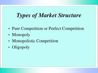
Discussion Topics • Market structure characteristics • Imperfect competition in selling • Imperfect competition in buying • Market structure in livestock industry • Governmental regulatory measures
Market Structure Characteristics • Number of firms and size distribution • Product differentiation • Barriers to entry • Picture here tells a tale of two markets (no. 2 yellow corn vs. farm equipment) Pages 145-146
Market Structure Characteristics • Number of firms and size distribution • Product differentiation • Barriers to entry • Existing economic environment (the conditions of supply and demand) Pages 145-146
Perfect Competition • Up to now we have been assuming the firm and market reflect the conditions of perfect competition… farmers come close as anybody to meeting these conditions. • A large number of small firms (2 million farms) • A homogeneous product (no. 2 yellow corn) • Freely mobile resources (no barriers to entry, no patents, for example, as well as no barriers to exit) • Perfect knowledge of market conditions (outlook information from government and university sources, for example, The Texas Agricultural Extension System or the U.S. Department of Agriculture)
Merging Demand and Supply Price D S Chapters 6,8 PE Chapters 3,4,5 Chapter 8 QE Quantity
Firm is a “Price Taker” Under Perfect Competition The Market The Firm Price Price D S AVC MC PE QE OMAX Quantity
If Demand Increases…… The Market The Firm D1 Price Price D S AVC MC PE QE 10 11 Quantity
If Demand Decreases…… The Market The Firm Price Price D S D2 AVC MC PE QE 9 10 Quantity
Firm is a “Price Taker” in the Input Market Labor Market The Firm Price Price D S MVP MIC PE QE LMAX Quantity
Firm is a “Price Taker” in the Input Market Labor Market The Firm Wage rate Price D S MVP MIC PE QE LMAX Quantity
Imperfect Competition • Many of the markets in which farmers buy inputs and sell their products however do not meet these conditions
Imperfect competitors selling a differentiated product have a downward sloping demand curve since now they can have an influence on price (e.g., they can differentiate product) (unlike perfectly competitive firms which have a perfectly elastic horizontal demand curve because they and buyers cannot influence price) Page 150
The marginal revenue in this instance also is downward sloping, and goes to zero at the point where total revenue peaks Page 150
Types of Imperfect Competitors on the Selling Side • Monopolistic competition • Oligopoly • Monopoly Let’s start here…
Monopolistic Competitors • Many sellers • Ability to differentiate product by advertising and sales promotions • Profits can exist in the short run, but others bid them away in the long run • Equate MC with MR, but price off the downward sloping demand curve Page 148-151
Short run profits. The firm produces QSR where MR=MC at E above, but prices its products at PSR by reading off the demand curve which reveals consumer willingness to pay Page 150
Short run loss. The firm suffers a loss in the current period following the same strategy of operating at QSR given by MC=MR at point E. Page 150
At quantity QSR, average total cost (ATCSR) is greater than PSR, which creates the loss depicted above… Page 150
In the long run, profits are bid away as more firms enter the market. Or losses will no longer exist as firms leave the market. At QLR, the remaining firms are just breaking even as shown by the lack of gap between the demand curve and ATC curve. Page 151
Top 10 Burger Restaurants Imperfect competition (monopolistic competition) you face weekly
Oligopolies • A few number of sellers, each of which is large enough to have influence on market volume and price • Non-price competition between oligopolists • Match price cuts but not price increases by fellow oligopolists • Like monopolistic competitors, they have some ability to set market prices Pages 152-155
Examples of Oligopolists • Farm machinery manufacturers • Domestic automobile industry • Domestic airline industry • Pesticide and fertilizer industry Products sold are largely identified or differentiated by company brand or name.
Demand curve DD represents the case when all oligopolists move prices together and share the market. Page 154
Demand curve dd represents the case when a single firm changes its price abovePe at point 1. This situation leads to a kinked demand curve d1D and a discontinuous marginal revenue curve. Note: dd is more elastic than DD Why? Rival oligopolists will match all price cuts but not all price increases in the short run because they want to maintain market share. Page 154
Meeting demand along the lower segment of the kinked demand curve, the firm is maintaining its market share. This situation also explains why there is a tendency for prices to remain at Pe Page 187
Note that shifting MC curves reflecting technological advances will not affect PE and QE. (MC drops from point 3 to point 4). This situation explains why oligopolistic markets are characterized by infrequent price changes. Firms usually do not change their price-quantity combinations in response to small shifts of their cost curves. Page 187
Monopoly (not the Parker Brothers Game) • Only seller in the market • Entry of other firms is restricted by patents, etc. • They have absolute power over setting market price • They produce a unique product • They can make economic profits in the long run because they can set price without competition. Page 155-158
Total revenue is equal to the area 0PECQE, which forms the blue box to the left… Notice the monopoly, like the previous forms of imperfect competition, produces where MC=MR (point A), but then reads up to the demand curve (point C) when setting price PE. Page 156
Total variable costs for the monopolist is equal to area 0NAQE, or the yellow box to the left. Page 156
Total fixed costs for the monopolist is equal to area NMBA, or the green box to the left… Page 156
Total cost is therefore equal to area 0MBQE, or the green box plus the yellow box to the left Page 156
Finally, the economic profit earned by the monopolist is equal to area MPECB, or total revenue (blue box) minus total costs (green box plus yellow box). Page 156
Let’s compare a monopoly with perfect competition from an economic welfare perspective Page 157
Perfect Competition Case Consumer surplus under perfect competition is equal to the sum of areas 1, 4, 5, 8 and 9, or the blue triangle to the left Page 157
Perfect Competition Case Producer surplus under perfect competition is equal to the sum of areas 2, 3, 6 and 7, or the green triangle to the left Page 157
Perfect Competition Case Total economic surplus under perfect competition is therefore equal to the blue and green triangles to the left, or the sum of areas 1 through 9. Page 157
Monopoly Case Consumer surplus under a monopoly is equal to the sum of areas 8 and 9, or the new blue triangle to the left Thus, consumers would be economically worse off by areas 1, 4 and 5 under a monopoly. They are paying a higher price PM and they are receiving a smaller quantity QM. Page 157
Monopoly Case Producer surplus under a monopoly is equal to the sum of areas 3, 4, 5, 6 and 7, or the green area to the left. Thus, producers lose area 2 but gain areas 4+5, making them economically better off than perfect competitors Page 157
Monopoly Case Finally, society as a whole would be economically worse off by areas 1+2. This magnitude of loss is called a dead weight loss. Dead weight loss may not necessarily be large. This measure reflects the cost to society due to the existence of a monopoly in lieu of perfect competition. Page 157
Summary of imperfect competitors from a selling perspective Page 157