Download
1 / 83
850 likes | 1.09k Views
Learn about the characteristics of perfect competition, price-taking behavior, revenue calculations, and optimal output levels in a perfectly competitive market. Explore the demand and marginal revenue curves, supply curves, short-run shutdown points, and graphing firm profits.

E N D
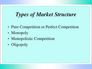
Types of Market Structure • Pure Competition or Perfect Competition • Monopoly • Monopolistic Competition • Oligopoly
Assumptions of Perfect Competition • Many independent firms • Each seller is small relative to the whole market • Homogeneous (identical) product • Easy entry and exit (no barriers to entry)
Price Taking The perfectly competitive firm is said to be a price-taker, because it takes the market price as given and has no control over the price. Why?...
If the firm tried to charge a higher price, it would lose all its business. Customers could go elsewhere to buy the same product for less. Since the firm is very small, it can sell as much as it wants at the market price. So there’s no reason to charge a lower price.
The demand curve for the product of the perfectly competitive firm shows how much can be sold at specific prices. Let’s see what it would look like... The firm can sell as little or as much as it wants at the market price. Suppose, for example, the market price is $5.
The firm can sell 10 units for $5. price $5 10 quantity
The firm can sell 20 units for $5. price $5 20 quantity
The firm can sell 30 units for $5. price $5 30 quantity
The firm can sell 40 units for $5. price $5 40 quantity
The firm can sell 50 units for $5. price $5 50 quantity
So all these points are on the demand curve for the firm’s product. price $5 quantity
Connecting these points, we have the demand curve for the firm’s product. price $5 demand quantity
The demand curve for the perfectly competitive firm’s product is a horizontal line at the market price. price market price demand quantity
Recall: Total Revenue Total Revenue = Price x Quantity TR = P Q
Recall: Marginal Revenue (MR) Marginal Revenue is the additional revenue earned from selling one additional unit of output. MR = DTR / DQ
comment For ease of writing, instead of writing the “perfectly competitive” firm we will frequently write the “p.c.” firm.
The MR Curve for the p.c. Firm For the p.c. firm, MR is equal to the market price. So MR is a horizontal line at the level of that price. The demand curve for the p.c. firm is also a horizontal line at the level of the market price. So, for the p.c. firm, the demand curve and the MR curve are the same horizontal line.
The demand curve (D) and the MR curve for the perfectly competitive firm’s product. price market price D = MR quantity
Optimal Output Level Recall: To maximize profit, the firm will produce at the output level where MR = MC. So the firm will produce where the MR and MC curves intersect.
Draw your axes; label them quantity and $. $ Quantity
Draw your ATC, AVC, and MC curves. (Make sure MC intersects ATC and AVC at the minimum.) $ ATC AVC MC Quantity
Draw the D = MR curve horizontal at the market price. $ D = MR ATC AVC MC Quantity
If the market price is P1 , the quantity produced will be Q1. $ D = MR P1 ATC AVC MC Quantity Q1
If the market price is P2 , the quantity produced will be Q2. $ ATC D = MR P2 AVC MC Quantity Q2
If the market price is P3 , the quantity produced will be Q3. $ ATC AVC P3 D = MR MC Quantity Q3
If the market price is P4 , the quantity produced will be Q4. $ ATC AVC P4 D = MR MC Quantity Q4
If the market price is P5 , the quantity produced will be Q5. $ ATC AVC D = MR P5 MC Quantity Q5
Price P5 was the minimum of the AVC curve (the shutdown point). If the price fell any lower than P5 the firm would produce no output.
The p.c. firm’s short run supply curve The firm’s supply curve shows the quantity the firm will produce at each price. The P, Q values we have shown, therefore, are points on the firm’s supply curve. But those points are all on the firm’s MC curve. So, the firm’s supply curve is the part of the MC curve that is above the minimum of the AVC curve.
The p.c. firm’s short run supply curve Supply $ ATC AVC MC Quantity
The market short run supply curve To determine the total amount that all the firms will produce at each price, we simply add up the amounts that each of the firms will produce at that price.
A little trick for graphing a firm’s profitRecall for a rectangle: Area = length . width length Area width
We also know TR = P . Q. So, if we can find a rectangle whose length is P and whose width is Q, then its area must be total revenue. P TR Q
To determine Total Cost, first remember ATC = TC / Q So, ATC.Q = TC
To determine Total Cost, first remember ATC = TC / Q So, ATC.Q = TC Now, if we can find a rectangle whose length is ATC and whose width is Q, then its area is TC. ATC TC Q
Then to determine profit, we just subtract the TC area from the TR area.
Step 1 a. Draw your axes and label them Q and $. ( Label the origin 0.) $ 0 Quantity
Step 1b. Draw the firm’s ATC curve. (If the price is below the minimum of ATC, you will also need to draw the AVC curve.) MC $ ATC P 0 Quantity
Step 1 c. Draw the MC curve and D=MR curve. (For a positive profit, D must be at least partly above ATC.) MC $ ATC P D = MR 0 Quantity
Step 2: Determine the profit-maximizing output (Q*) by finding where MR = MC. MC $ ATC P D = MR 0 Quantity Q*
Step 3: Find your TR = PQ rectangle. MC ATC $ P D = MR 0 Quantity Q*
Step 4: Determine ATC at the profit-maximizing output level. MC ATC $ P D = MR ATC 0 Quantity Q*
Step 5: Find your TC = ATC . Q rectangle. MC ATC $ P D = MR Quantity Q*
Step 6: Find profit p = TR - TC. MC ATC $ P p r o f i t D = MR Quantity Q*
You follow the same steps to draw a firm that is making a loss or breaking even (zero profits).Let’s do a firm with a loss.
Step 1: Draw & label the curves & axes. For a loss, put D above the minimum of AVC & below the minimum of ATC. MC $ ATC AVC P D = MR 0 Quantity
Step 2: Determine the profit-maximizing output (Q*) by finding where MR = MC. MC $ ATC AVC P D = MR 0 Quantity Q*