Network Flow
Network Flow. What is a network? Flow network and flows Ford-Fulkerson method - Residual networks - Augmenting paths - Cuts of flow networks Max-flow min-cut theorem. Chapter 26: Maximum Flow. A directed graph is interpreted as a flow network:


Network Flow
E N D
Presentation Transcript
Network Flow • What is a network? • Flow network and flows • Ford-Fulkerson method - Residual networks - Augmenting paths - Cuts of flow networks • Max-flow min-cut theorem
Chapter 26: Maximum Flow • A directed graph is interpreted as a flow network: - A material coursing through a system from a source, where the material is produced, to a sink, where it is consumed. - The source produces the material at some steady rate, and the sink consumes the material at the same rate. • Maximum problem: to compute the greatest rate at which material can be shipped from the source to the sink.
Edmonton Saskatoon Capacity 12 16 20 Vancouver Winnipeg 9 4 10 7 v1 v2 v3 v4 v2 v1 v3 v4 4 13 t t s s 14 Calgary Regina • Example Edmonton Saskatoon Capacity 12 0 16 20 Vancouver Winnipeg 9 0 4 10 0 0 7 0 0 0 4 13 0 14 Calgary Regina
Applications which can be modeled by the maximum flow - Liquids flowing through pipes - Parts through assembly lines - current through electrical network - information through communication network
Definition – flow networks and flows - A flow network G = (V,E) is a directed graph in which each edge (u, v) E has a nonnegative capacity c(u,v) 0. - source: s; sink: t - For every vertex v V, there is a path: s ↝ v ↝ t - A flow in G is a real-valued function f: V V Rthat satisfies the following properties: Capacity constraint: For all u, v V, f(u, v) c(u, v). Skew symmetry: For all u, v V, f(u, v) = - f(v, u). Flow conservation: For all u V – {s, t}, = 0.
v1 v2 v3 v4 s t The quantity f(u,v), which can be positive, zero, or negative, is called the flow from vertex u to vertex v. The value of a flow f is defined as the total flow out of the source |f| = • Example Edmonton Saskatoon 12/12 15/20 11/16 Vancouver Winnipeg 4/9 7/7 1/4 -1/10 4/4 8/13 11/14 Calgary Regina
v1 v2 v3 v4 s t = 0. The total flow out of a vertex is 0. • Example Edmonton Saskatoon 12/12 -12/0 15/20 11/16 Vancouver 4/9 Winnipeg -11/0 -15/0 -1/10 1/4 7/7 -7/0 -4/0 -4/0 -8/0 4/4 8/13 -11/0 11/14 Calgary Regina = 0. The total flow into a vertex is 0.
The total positive flow entering a vertex v is defined by The total net flow at a vertex is the total positive flow leaving the vertex minus the total positive flow entering the vertex. The interpretation of the flow-conservation property: • The total positive flowing entering a vertex other than the source or sink must equal the total positive flow leaving that vertex. • For all u V – {s, t}, = 0. That is, the total flow out of u is 0. For all v V – {s, t}, = 0. That is, the total flow into v is 0.
10 s1 t2 s1 s3 s4 s5 t1 s2 s2 t3 t2 t1 t3 s5 s4 s3 3 10 t ∞ 12 3 ∞ 12 15 5 ∞ 6 15 5 8 ∞ ∞ 6 s 14 8 20 ∞ ∞ 14 7 20 ∞ 13 7 11 13 11 18 2 18 2 • Networks with multiple sources and sinks - Introduce supersource s and supersinkt
Working with flows - implicit summation notation f(X, Y) = The flow-conservation constraint can be re-expressed as f(u, V) = 0 for all u V – {s, t}. - Lemma 26.1 Let G = (V, E) be a flow network, and let f be a flow in G. Then, the following equalities hold: 1. For all X V, we have f(X, X) = 0. 2. For all X, Y V, we have f(X, Y) = - f(Y, X). 3. For all X, Y, Z V with X Y = ø, we have the sums f(X Y, Z) = f(X, Z) + f(Y, Z), f(Z, X Y) = f(Z, X) + f(Z, Y).
Working with flows - |f| = f(V, t) |f| = f(s, V) = f(V, V) – f(V – s, V) = - f(V – s, V) = f(V, V – s) = f(V, t) + f(V, V – s – t) = f(V, t)
The Ford-Fulkerson method - The maximum-flow problem: given a flow network G with source s and sink t, we wish to find a flow f of maximum value. ( ) - important concepts: residual networks augmenting paths cuts Ford-Fulkerson-Method(G, s, t) 1. Initialize flow f to 0 2. while there exists an augmenting path p 3. do augment flow f along p 4. returnf
Residual networks - Given a flow network and a flow, the residual network consists of edges that can admit more flow. - Let f be a flow in G = (V, E) with source s and sink t. Consider a pair of vertices u, v V. The amount of additional flow we can push from u to v before exceeding the capacity c(u, v) is the residual capacity of (u, v), given by cf(u, v) = c(u, v) – f(u, v). - Example If c(u, v) = 16 and f(u, v) = 11, then cf(u, v) = 16 – 11 = 5. If c(u, v) = 16 and f(u, v) = -4, then cf(u, v) = 16 – (-4) = 20.
v1 v2 v3 v4 s t • Residual networks - Given a flow network G = (V, E) and a flow f, the residual network of G induced by f is Gf= (V, Ef), where Ef = {(u, v) V V: cf(u, v) > 0}. - Example Edmonton Saskatoon 12/12 -12/0 15/20 11/16 Vancouver 4/9 Winnipeg -11/0 -15/0 -1/10 1/4 7/7 -7/0 -4/0 -4/0 -8/0 4/4 8/13 -11/0 11/14 Calgary Regina
v1 v2 v3 v4 s t • Residual networks residual network: Edmonton Saskatoon 0 12 5 5 Vancouver Winnipeg 11 5 15 11 3 0 7 4 8 4 0 5 11 3 Calgary Regina |Ef| 2|E|
Residual networks Lemma 26.2 Let G = (V, E) be a network with source s and sink t, and let f be a flow in G. Let Gf be the residual network of G induced by f, and let f’ be a flow in Gf.Then, the flow sum f + f’ (defined by (f + f’ )(u, v) = f (u, v) + f’ (u, v)) is a flow in G with value |f + f’| = |f | + |f’|. Proof. We must verify that skew symmetry, the capacity constraints, and flow conservation are obeyed. skew symmetry: (f + f’)(u, v) = f (u, v) + f’(u, v) = - f (v, u) - f’(v, u) = - (f (v, u) + f’(v, u)) = - (f + f’)(v, u).
capacity constraint: (f + f’)(u, v) = f (u, v) + f’(u, v) f (u, v) + (c(u, v) - f(u, v)) = c(u, v). flow conservation: = = + = 0 + 0 = 0. Finally, we have |f + f’| = = = + = |f |+ |f’|
v1 v2 v3 v4 s t • Augmenting paths - Given a flow network G = (V, E) and a flow f, an augmenting path p is a simple path from s to t in the residual network Gf. - Example Edmonton Saskatoon 12 5 5 Vancouver Winnipeg 11 5 15 11 3 7 4 8 4 5 11 3 Calgary Regina
Augmenting paths - In the above residual network, path s v2 v3 t is an augmenting path. - We can increase the flow through each edge of this path by up to 4 units without violating a capacity constraint since the smallest residual capacity on this path is cf(v2, v3) = 4. - residual capacity of an augmenting path cf(p) = min{cf(u, v): (u, v) is on p}. - Lemma 26.3 Let G = (V, E) be a network, let f be a flow in G, and let p be an augmenting path in Gf. Define a function fp: V V R by cf(p) if (u, v) is on p, fp(u, v) = - cf(p) if (v, u) is on p, 0 otherwise. Then, fp is a flow in Gf with value |fp| = cf(p).
- Example Edmonton Saskatoon 12/12 v3 v1 11/16 -12/0 15/20 Vancouver Winnipeg 4/9 -11/0 -15/0 s t -1/10 1/4 7/7 -7/0 -4/0 -4/0 -8/0 4/4 8/13 -11/0 v2 v4 11/14 Calgary Regina Edmonton Saskatoon 12/12 v1 v3 -12/0 11/16 19/20 Winnipeg Vancouver 0/9 -11/0 -19/0 s t -1/10 1/4 7/7 -7/0 -4/0 0/0 -12/0 4/4 -11/0 12/13 v2 v4 11/14 Calgary Regina
v1 v2 v3 v4 s t - Residual network induced by the new flow Edmonton Saskatoon 0 12 1 5 Vancouver Winnipeg 11 9 19 11 3 0 7 4 12 0 0 1 11 3 Calgary Regina
Augmenting paths - Corollary 26.4Let G = (V, E) be a network, let f be a flow in G, and let p be an augmenting path in Gf. Let fp be defined as in Lemma 26.3. Define a function f’: V V R by f’ = f + fp. Then, f’ is a flow in G with value | f’| = |f | + |fp| > |f |. Proof. Immediately from Lemma 26.2 and 26.3. • Ford-Fulkerson Algorithm - The Ford-Fulkerson method repeatedly augments the flow along augmenting paths until a maximum flow has been found. - A flow is maximum if and only if its residual network contains no augmenting path.
Ford-Fulkerson algorithm Ford_Fulkerson(G, s, t) 1. for each edge (u, v) E(G) 2. dof(u, v) 0 3. f(v, u) 0 4. while there exists a path p from s to t in Gf 5. docf(p) min{cf (u, v) : (u, v) is in p} 6. for each edge (u, v) on p 7. dof(u, v) f(u, v) + cf(p) 8. f(v, u) - f(u, v)
0/12 0/16 0/20 v1 v2 v4 v3 v2 v4 v3 v1 0/9 0/4 0/10 0/7 0/4 t s t s 0/13 0/14 • Sample trace Initially, the flow on edge is 0. The corresponding residual network: 12 16 20 9 4 10 7 4 13 14
v1 v2 v3 v4 v4 v3 v2 v1 t t s s • Sample trace Pushing a flow 4 on p1(an augmenting path) 4/12 4/16 0/20 4/9 0/4 0/10 0/7 4/4 0/13 4/14 The corresponding residual network: 8 12 20 4 5 4 10 4 7 4 4 0 4 13 10
v1 v1 v2 v3 v4 v4 v3 v2 s t t s • Sample trace Pushing a flow 7 on p2(an augmenting path) 4/12 11/16 7/20 4/9 -7/4 7/10 7/7 4/4 0/13 11/14 The corresponding residual network: 8 5 13 4 5 7 11 3 11 7 0 4 4 0 11 13 3
v2 v1 v2 v3 v4 v4 v3 v1 s t s t • Sample trace Pushing a flow 8 on p3(an augmenting path) 12/12 11/16 15/20 4/9 1/4 -1/10 7/7 4/4 8/13 11/14 The corresponding residual network: 0 5 5 12 5 15 3 11 11 7 0 4 8 4 0 11 5 3
v3 v1 v2 v3 v4 v4 v2 v1 s t s t • Sample trace Pushing a flow 4 on p4(an augmenting path) 12/12 11/16 19/20 0/9 1/4 -1/10 7/7 0/0 4/4 12/13 11/14 The corresponding residual network: no augmenting paths! 0 5 1 12 9 19 3 11 11 7 0 4 12 0 0 11 1 3
Analysis of Ford-Fulkerson algorithm In practice, the maximum-flow problem often arises with integral capacities. If the capacities are rational numbers, an appropriate scaling transformation can be used to make them all integral. Under this assumption, a straightforward implementation of Ford-Fulkerson algorithm runs in time O(E|f*|), where f* is the maximum flow found by the algorithm. The analysis is as follows: 1. Lines 1-3 take time (E). 2. The while-loop of lines 4-8 is executed at most |f*| times since the flow value increases by at least one unit in each iteration. Each iteration takes O(E) time.
v1 v2 s 12/12 v3 15/20 11/16 4/9 7/7 1/4 -1/10 t 4/4 8/13 v4 11/14 • Cuts of flow networks - A cut (S, T) of flow network G = (V, E) is a partition of V into S and T = V – S such that s S and t T. - netflow across the cut (S, T) is defined to be f(S, T). f({s, v1, v2}, {v3, v4, t}) = f(v1, v3) + f(v2, v3) + f(v2, v4) = 12 + (-4) + 11 = 19. The net flow across a cut (S, T) consists of positive flows in both direction. 30
v1 v2 s • Cuts of flow networks - The capacity of the cut (S, T) is denoted by c(S, T), which is computed only from edges going from S to T. 12/12 v3 15/20 11/16 4/9 7/7 1/4 -1/10 t 4/4 8/13 v4 11/14 c({s, v1, v2}, {v3, v4, t}) = c(v1, v3) + c(v2, v4) = 12 + 14 = 26. 31
Cuts of flow networks - The following lemma shows that the net flow across any cut is the same, and it equals the value of the flow. Lemma 26.5 Let f be a flow in a flow network G with source s and sink t, and let (S, T) be a cut of G. Then, the net flow across (S, T) is f(S, T) = |f|. Proof. Note that f(S – s, V) = 0 by flow conservation. So we have f(S, T) = f(S, V - S) = f(S, V) - f(S, S) = f(S, V) = f(s, V) + f(S – s, V) = f(s, V) = |f|.
Cuts of flow networks - Corollary 26.6 The value of any flow in a flow network G is bounded from above by the capacity of any cut of G. Proof. |f| = f(S, T) = = c(S, T).
Max-flow min-cut theorem Theorem 26.7 If f is a flow network G = (V, E) with source s and sink t, then the following conditions are equivalent: 1. f is a maximum flow in G. 2. The residual network Gf contains no augmenting paths. 3. |f| = c(S, T) for some cut (S, T) of G. Proof. (1) (2): Suppose for the sake of contradiction that f is a maximum flow in G but that Gf has an augmenting path p. Then, by Corollary 26.4, the flow sum f + fp, where fp is given by Lemma 26.3, is a flow in G with value strictly greater than |f|, contradicting the assumption that f is a maximum flow.
Max-flow min-cut theorem Theorem 26.7 If f is a flow network G = (V, E) with source s and sink t, then the following conditions are equivalent: 1. f is a maximum flow in G. 2. The residual network Gf contains no augmenting paths. 3. |f| = c(S, T) for some cut (S, T) of G. Proof. (2) (3): Suppose that Gf has no augmenting path. Define S = {v V: there exists a path from s to v in Gf} and T = V – S. The partition (S, T) is a cut: we have s S trivially and t S because there is no path from s to t in Gf. For each pair of vertices u and v such that u S and v T, we have f(u, v) = c(u, v), since otherwise (u, v) Ef, which would place v in set S. By Lemma 26.5, therefore, |f| = f(S, T) = c(S, T).
Max-flow min-cut theorem Theorem 26.7 If f is a flow network G = (V, E) with source s and sink t, then the following conditions are equivalent: 1. f is a maximum flow in G. 2. The residual network Gf contains no augmenting paths. 3. |f| = c(S, T) for some cut (S, T) of G. Proof. (3) (1): By Corollary 26.6, |f| c(S, T) for all cuts (S, T). The condition |f| = c(S, T) thus implies that f is a maximum flow.