Download
1 / 49
490 likes | 655 Views
Understand the significance of early exercise in option pricing to optimize decision-making. Explore put-call parity, dividend impact, and risk-neutral pricing concepts to enhance financial strategies and maximize returns in stock options.

E N D
Chapter 11 Binomial Option Pricing: II
Understanding Early Exercise • Options may be rationally exercised prior to expiration. • By exercising a Call option, the option holder • receives the stock and thus receives dividends, • pays the strike price prior to expiration (this has an interest cost), • loses the insurance/flexibility implicit in the call.
Understanding Early Exercise • By exercising a Put option, the option holder • receives the strike price and thus collects interest on it going forward, • gives the stock away and thus stops receiving dividends • loses the insurance/flexibility implicit in the put.
Call Option Without Dividends • Put-Call Parity says: C=P+S-Ke-rT • Since P>0, C>S-Ke-rT • And since K>Ke-rT , we have C>S-K • Therefore the Call price C is always greater than the intrinsic value S-K (which is what you would get if you exercised). • Thus it is never optimal to exercise an American Call option on a non-dividend paying stock!!!
Call Option With Dividends • Put-Call Parity says: C=P+S-Ke-rT-D • (where D is the present value of all future dividends to be received) • So C = S-K + P + K-Ke-rT – D • Thus C = S-K + P + K(1-e-rT) – D • Therefore, when S is high and thus P close to zero, the Call price C can be greater or lower than the intrinsic value S-K (which is what you would get if you exercised) depending on whether K(1-e-rT) is greater or lower than D, i.e. whether the interest saved by delaying the payment K is greater or lower than the lost dividends. • Thus it can be optimal to exercise an American Call option on a dividend-paying stock.
Put Option Without Dividends • Put-Call Parity says: P=C+Ke-rT-S • Thus P = K-S + C-K(1-e-rT) • Therefore the Put price P can be greater or lower than the intrinsic value K-S depending on whether C is greater or lower than K(1-e-rT). • Thus even on a non-dividend paying stock, it may be optimal to exercise a Put option ! (It usually happens for low values of S, when C is very small)
Understanding Risk-Neutral Pricing • A risk-neutral investor is indifferent between a sure thing and a risky bet with an expected payoff equal to the value of the sure thing. • p* is the risk-neutral probability that the stock price will go up. • The option pricing formula can be said to price options as if investors are risk-neutral. • Note that we are not assuming that investors are actually risk-neutral, and that risky assets are actually expected to earn the risk-free rate of return.
Pricing an option using risk-neutral probabilities • Consider a world populated by risk-neutral investors. • Investors would only be concerned with expected returns, and not about the level of risk. • Hence investors would not “charge” or require a premium for risky securities. • Therefore risky securities would have the same expected rate of return as riskless securities. In other words, every security is returning the risk-free rate.
Fine point to think about: • Now consider the following scenario: suppose a risky security is expected to achieve great growth and great future profits. (You can even assume that the security actually delivers on its promises later, if you wish.) • Even though risk-neutral investors might only usually require the risk-free rate of return, doesn’t this mean that the expected rate of return on this security will be much higher than the risk-free rate? And if yes, doesn’t that invalidate what we’ve just discussed? • WHAT IS GOING ON HERE ? ANY POSSIBLE RECONCILIATION OF THE TWO IDEAS?
Pricing an option using risk-neutral probabilities • If the stock is thus expected to earn the risk-free rate r and pays out a continuous dividend yield d, then the risk-neutral probability p* that the stock will go up must satisfy: p*u edhS + (1 – p*)d edhS = erhS • Solving for p* gives us
Pricing an option using real probabilities • Is option pricing consistent with standard discounted cash flow calculations? Yes. However, discounted cash flow is not used in practice to price options. • This is because it is necessary to compute the option price in order to compute the correct discount rate.
Pricing an option using real probabilities • Suppose that the continuously compounded expected return on the stock is and that the stock does not pay dividends. • If p is the true probability of the stock going up, p must be consistent with u, d, and : puS + (1 – p)dS = ehS (11.3) • Solving for p gives us (11.4)
Pricing an option using real probabilities • Using p, the actual expected payoff to the option one period hence is (11.5) • At what rate do we discount this expected payoff? • It is not correct to discount the option at the expected return on the stock, , because the option is equivalent to a leveraged investment in the stock and hence is riskier than the stock.
Pricing an option using real probabilities • Let us denote the appropriate per-period discount rate for the option as . • Since an option is equivalent to holding a portfolio consisting of shares of stock and B bonds, the expected return on this portfolio is (11.6) • And since an option is equivalent to holding a portfolio consisting of shares of stock and B bonds, the denominator is indeed the option price. This confirms that in order to compute the discount rate g, one needs to have the price of the option first.
Pricing an option using real probabilities • We can nevertheless now compute the option price as the expected option payoff, discounted at the appropriate discount rate, given by equation (11.6). We thus need to compute: (11.7) • It turns out that this gives us the same option price as performing the risk-neutral calculation.
Application: one-period example • Assume the following information: • a=15%, S=$41, K=$40, s=30%, r=8%, T=1, h=1, and d=0. The “up-price” for the stock is $59.954 and the “down-price” is $32.903. • Compute the price of a European call option by using: • True probabilities • Risk-neutral probabilities Are the results identical?
Application: one-period example • The true up probability is (with u = 59.954 / 41 = 1.4623 and d = 32.903 / 41 = 0.8025): • p = [e0.15-0.8025] / [1.4623-0.8025] = 0.5446. • The expected option payoff therefore is: • 0.5446($19.954) + (1-0.5446)($0) = $10.867 • We now need to compute the discount rate g in order to get the option price today.
Application: one-period example • For g, we need the values of D and B. • D = (19.954-0)/(59.954-32.903) = 0.738 • B is the present value of loan needed to match cash flows of DS and option (pick the case where stock goes down, since easier – but works for both): • B = -e-0.08[(0.738)(32.903)-0] = - $ 22.405 • We thus have: • Or g = ln(1.386) = 32.64%
Application: one-period example • Finally, armed with g, we can compute the discounted expected option value as: • C = e-.3264(10.867) = $ 7.839
Application: one-period example • The risk-neutral probability of the stock going up is: • p* = [e0.08-0.8025] / [1.4623-0.8025] = 0.4256. • The call option price therefore is: • C = e-0.08[(0.4256)(19.954)+(1- 0.4256)(0)] = $ 7.839 • This is exactly the price we obtained before.
The Binomial Tree and Lognormality • The usefulness of the binomial pricing model hinges on the binomial tree providing a reasonable representation of the stock price distribution. • The binomial tree approximates a lognormal distribution.
The random walk model • It is often said that stock prices follow a random walk. • Imagine that we flip a coin repeatedly. • Let the random variable Y denote the outcome of the flip. • If the coin lands displaying a head, Y = 1; otherwise, Y = – 1. • If the probability of a head is 50%, we say the coin is fair. • After n flips, with the ith flip denoted Yi, the cumulative total, Zn, is (11.8) • It turns out that the more times we flip, on average the farther we will move from where we started.
The random walk model • We can represent the process followed by Znin term of the change in Zn: Zn – Zn-1 = Yn or Heads: Zn – Zn-1 = +1 Tails: Zn – Zn-1 = –1
The random walk model • A random walk, where with heads, the change in Z is 1, and with tails, the change in Z is – 1:
The random walk model • The idea that asset prices should follow a random walk was articulated in Samuelson (1965). • In efficient markets, an asset price should reflect all available information. In response to new information the price is equally likely to move up or down, as with the coin flip. • The price after a period of time is the initial price plus the cumulative up and down movements due to new information.
Modeling prices as a random walk. • The above description of a random walk is not a satisfactory description of stock price movements. There are at least three problems with this model: 1. If by chance we get enough cumulative down movements, the stock price will become negative. 2. The magnitude of the move ($1) should depend upon how quickly the coin flips occur and the level of the stock price. 3. The stock, on average, should have a positive return. However, the random walk model taken literally does not permit this. • The binomial model is a variant of the random walk model that solves all of these problems.
Continuously compounded returns • The binomial model assumes that continuously compounded returns are a random walk. • Some important properties of continuously compounded returns: • The logarithmic function computes returns from prices. • The exponential function computes prices from returns. • Continuously compounded returns are additive. • Continuously compounded returns can be less than –100%.
The standard deviation of returns • Suppose the continuously compounded return over month i is rmonthly,i. The annual return is • The variance of the annual return is (11.14)
The standard deviation of returns • Suppose that returns are uncorrelated over time and that each month has the same variance of returns. Then from equation (11.14) we have 2 = 12 2monthly , where 2 is the annual variance. The annual standard deviation is • If we split the year into n periods of length h (so that h = 1/n), the standard deviation over the period of length h is (11.15)
The binomial model • The binomial model is • Taking logs, we obtain (11.16) • Since ln (St+h/St) is the continuously compounded return from t to t+h, the binomial model is simply a particular way to model the continuously compounded return. • That return has two parts, one of which is certain, (r–)h, and the other of which is uncertain, h.
The binomial model • Equation (11.6) solves the three problems in the random walk: 1. The stock price cannot become negative. 2. As h gets smaller, up and down moves get smaller. 3. There is a (r – )h term, and we can choose the probability of an up move, so we can guarantee that the expected change in the stock price is positive.
Lognormality and the binomial model • The binomial tree approximates a lognormal distribution, which is commonly used to model stock prices. • The lognormal distribution is the probability distribution that arises from the assumption that continuously compounded returns on the stock are normally distributed. • With the lognormal distribution, the stock price is positive, and the distribution is skewed to the right, that is, there is a chance of extremely high stock prices.
Lognormality and the binomial model • The binomial model implicitly assigns probabilities to the various nodes.
Lognormality and the binomial model • The following information is used to draw the graphs on the next slides: initial stock price S = 100, s=30%, E(RS)=10%, T=1year, and we divide the 1-year period into 25 periods (h=1/25). Note that n=25. • The probability of the stock going up from one period to the next is p=[eRh-d]/[u-d] • Use u=es sqrt(h) and d=e-s sqrt(h) . • Proba of reaching ith node =(number of ways to reach ith node) pn-i(1-p)i where number of ways to reach the ith node = n!/[(n-i)!i!]
Lognormality and the binomial model • The following graph compares the probability distribution for a 25-period binomial tree with the corresponding lognormal distribution:
Lognormality and the binomial model: Exercise • Use the following information to draw a probability distribution graph: initial stock price S = 100, s=30%, E(RS)=10%, T=1year, and we divide the 1-year period into 3 periods (h=1/3). Note that therefore n=3. • The probability of the stock going up from one period to the next is: p=[eRh-d]/[u-d] • Use u=essqrt(h) and d=e-s sqrt(h) . • The probability of reaching the ith node = (number of ways to reach the ith node) x pn-i(1-p)i where the number of ways to reach the ith node = n!/[(n-i)!i!]
Alternative binomial trees • There are other ways besides equation (11.6) to construct a binomial tree that approximates a lognormal distribution. • An acceptable tree must match the standard deviation of the continuously compounded return on the asset and must generate an appropriate distribution as h 0. • Different methods of constructing the binomial tree will result in different u and d stock movements. • No matter how we construct the tree, to determine the risk-neutral probability, we use and to determine the option value, we use C = e–rh [p* Cu + (1 – p*) Cd]
Alternative binomial trees • The Cox-Ross-Rubinstein binomial tree: • The tree is constructed as (11.18) • A problem with this approach is that if h is large or is small, it is possible that erh > eh. In this case, the binomial tree violates the restriction of u > e(r–)h > d. • In practice, h is usually small, so the above problem does not occur.
Alternative binomial trees • The lognormal tree: • The tree is constructed as (11.19) • Although the three different binomial models give different option prices for a finite number n, as n all three binomial trees converge to the same option price.
Is the binomial model realistic? • The binomial model is a form of the random walk model, adapted to modeling stock prices. The lognormal random walk model here assumes that • volatility is constant, • “large” stock price movements do not occur, • returns are independent over time. • All of these assumptions appear to be violated in the data.
Stock Paying Discrete Dividends • Suppose that a dividend will be paid between times t and t+h and that its future value at time t+h is D. • The time t forward price for delivery at t+h is Ft,t+h = St erh – D • Since the stock price at time t+h will be ex-dividend, we create the up and down moves based on the ex-dividend stock price: (11.20)
Stock Paying Discrete Dividends • When a dividend is paid, we have to account for the fact that the stock earns the dividend. (Sut + D) + erh B = Cu (Sdt + D) + erh B = Cd • The solution is • Because the dividend is known, we decrease the bond position by the PV of the certain dividend.
Problems with the discrete dividend tree 1. The conceptual problem with equation (11.20) is that the stock price could in principle become negative if there have been large downward moves in the stock prior to the dividend. But it is not an issue in reality since no firm would pay a large dividend if the stock is near zero, obviously. 2. The more practical problem is that the tree does not completely recombine after a discrete dividend is paid. The following tree is an example illustrating the issue:
A binomial tree using the prepaid forward • Hull (1997) presents a method of constructing a tree for a dividend-paying stock that solves both problems. • If we know for certain that a stock will pay a fixed dividend, then we can view the stock price as being the sum of two components: 1. the dividend, which is like a zero-coupon bond with zero volatility, and 2. the PV of the ex-dividend value of the stock, i.e., the prepaid forward price.
A binomial tree using the prepaid forward • Suppose we know that a stock will pay a dividend D at time TD < T, where T is the expiration date of the option. • We base the stock price movements on the prepaid forward price • This approach removes the shock associated with the dividend being paid, similar to the clean price of a bond smoothing the impact of a coupon payment shock. • As usual, the up and down movements are: • However, the actual stock price at each node is given by