Download
1 / 19
210 likes | 333 Views
This document explores the extraction of risk-neutral densities from option prices via mixture binomial trees. It outlines the motivation behind using market prices of traded options to understand market expectations for decision-making in areas such as exotic option pricing and risk measurement. The paper introduces mixture binomial trees for density extraction and discusses optimization methods, graphical modeling, and the implications of density extraction over time. Through applications on data from S&P 500 futures options, the study illustrates the value of risk-neutral probability assessments in trading.

E N D
Extracting Risk-Neutral Densities from Option Pricesusing Mixture Binomial Trees Christian Pirkner Andreas S. Weigend Heinz Zimmermann Version 1.0
Introduction Model Application Part 1 Part 2 Part 3 ü Outline • Motivation • Butterfly-Spread • Implied Binomial Tree Introduction • Mixture Binomial Tree • Optimization • Graph Model • Density Extraction: 1 Day • Density Extraction over Time • Conclusion Application
Introduction 1. Introduction Model - Motivation - Application • Goal: • What can we learn from market prices of traded options? Extract expectations of market participants • Use this information for decision making! Exotic option pricing, risk measurement and trading • An European equity call option (C) is the right to … • buy • an underlying security, S • for a specified strike price, X • at time to expiration, T payoff function: max [ST - X, 0]
X C Costbsp Payoff if ST = ... DC D(DC) 7 8 9 10 11 12 13 Buy 1 C(X=9) Sell 2 C(X=10) Buy 1 C(X=11) 7 3.354 -0.895 8 2.459 0.106 -0.789 9 1.670 +1.670 0 0 0 1 2 3 4 0.164 -0.625 10 1.045 -2.095 0 0 0 0 -2 -4 -6 0.184 -0.441 11 0.604 +0.604 0 0 0 0 0 1 2 0.162 -0.279 12 0.325 0.118 -0.161 13 0.164 0 0 0 1 0 0 0 Introduction 1. Introduction Model - … a butterfly-spread - Application vj 0.184 S=10
X C D(DC) Valuing an option with payoffs jusing vj: vj 7 3.354 Buying all vj’s: riskless investment 8 2.459 0.106 9 1.670 0.164 Defining Pj’s: “risk-neutral probabilities”: 10 1.045 0.184 11 0.604 0.162 Alternative way to value derivative: 12 0.325 0.118 13 0.164 Introduction 1. Introduction Model - … risk-neutral probabilities - Application S=10
Parametric • Linear • Logit • Polynomial • Gauss • Gamma • Edgeworth expansion • Smoothness • Mixture models • Several tanh Non Parametric • Kernel regression • Kernel density Introduction 1. Introduction Model - Density extraction techniques - Application II. Estimating density directly I. 2nd Derivative of call price function III. Recovering parameters of assumed stochastic process of the underlying security.
Introduction 1. Introduction Model - Standard & implied trees - Application • Instead of building a ... standard binomial tree • starting at time t=0 • resting on the assumption of normally distributed returns and constant volatility • We build an …implied binomial tree: • starting at time T • and flexible modeling of end-nodal probabilities
Subject to constraint: The weights of all mixture components are positive and add up to one ü Introduction 2. Model Model - Mixture binomial tree - Application … where we optimize for the lowest absolute mean squared error in option prices We propose to model end-nodal probabilities with a mixture of Gaussians ...
ü Introduction 2. Model Model - Mixture binomial tree - Application
ü Introduction 3. Application ü Model - Data: S&P 500 futures options - Application
ü Introduction 3. Evaluation & Analysis ü Model - February 6, 1 Gauss & Error - Application
ü Introduction 3. Evaluation & Analysis ü Model - February 6, 3 Gauss & Error - Application
ü Introduction 3. Evaluation & Analysis ü Model - February - Application
ü Introduction 3. Evaluation & Analysis ü Model - May - Application
ü Introduction 3. Evaluation & Analysis ü Model - July - Application
ü Introduction 3. Evaluation & Analysis ü Model - August - Application
ü Introduction 3. Evaluation & Analysis ü Model - October - Application
ü Introduction 3. Evaluation & Analysis ü Model - January - Application
ü Introduction Conclusion ü Model ü Application • Learning from option prices Extracting market expectations • Use information for decision making • Exotic option pricing Use extracted kernel to price non-standard derivatives: consistent with liquid options • Risk measurement Calculate “Economic Value at Risk” • Trading Take positions if extracted density differs from own view