Download
1 / 16
160 likes | 194 Views
Explore lossy audio compression methods such as LPC and CELP based on psychoacoustic models in MPEG Audio Layer I, II, and III, and understand human hearing sensitivity to different frequencies.

E N D
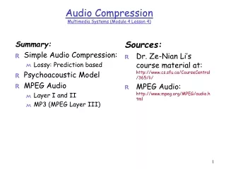
Summary: Simple Audio Compression: Lossy: Prediction based Psychoacoustic Model MPEG Audio Layer I and II MP3 (MPEG Layer III) Sources: Dr. Ze-Nian Li’s course material at:http://www.cs.sfu.ca/CourseCentral/365/li/ MPEG Audio:http://www.mpeg.org/MPEG/audio.html Audio Compression Multimedia Systems (Module 4 Lesson 4)
Simple Audio Compression Methods • Silence Compression - detect the "silence", similar to run-length coding • Adaptive Differential Pulse Code Modulation (ADPCM) e.g., in CCITT G.721 -- 16 or 32 Kbits/sec. • Encode the difference between two or more consecutive signals; the difference is then quantized --> hence the loss • Adaptive quantization • It is necessary to predict where the waveform is headed • Apple has proprietary scheme called ACE/MACE. A Lossy scheme that tries to predict where wave will go in next sample. Gives about 2:1 compression. • Linear Predictive Coding (LPC) fits signal to speech model and then transmits parameters of model. It sounds like a computer talking, 2.4 kbits/sec. • Code Excited Linear Predictor (CELP) does LPC, but also transmits error term --> audio conferencing quality at 4.8 kbits/sec.
Psychoacoustic Model Human hearing and voice • Frequency range is about 20 Hz to 20 kHz, most sensitive at 1 to 5 KHz. • Dynamic range (quietest to loudest) is about 96 dB • Normal voice range is about 500 Hz to 2 kHz • Low frequencies are vowels and bass • High frequencies are consonants How sensitive is human hearing? To answer this question we look at the following concepts: • Threshold of hearing Describes the notion of “quietness” • Frequency Masking A component (at a particular frequency) masks components at neighboring frequencies. Such masking may be partial. • Temporal Masking When two tones (samples) are played closed together in time, one can mask the other.
Threshold of hearing Experiment: Put a person in a quiet room. Raise level of 1 kHz tone until just barely audible. Vary the frequency and plot 40 30 bB 20 10 0 16 4 6 10 12 14 2 8 Frequency (KHz) • The ear is most sensitive to frequencies between 1 and 5 kHz, where we can actually hear signals below 0 dB. • Two tones of equal power and different frequencies will not be equally loud. • Sensitivity decreases at low and high frequencies.
Frequency Masking Experiment: Play 1 kHz tone (masking tone) at fixed level (60 dB). Play test tone at a different level (e.g., 1.1 kHz), and raise level until just distinguishable. Vary the frequency of the test tone and plot the threshold when it becomes audible:
Frequency Masking (Contd.) • Repeat previous experiment for various frequencies of masking tones
Temporal Masking • If we hear a loud sound, and then it stops, it takes a little while until we can hear a soft tone nearby (in frequency). • Experiment: • Play 1 kHz masking tone at 60 dB, plus a test tone at 1.1 kHz at 40 dB. Test tone can't be heard (it's masked). • Stop masking tone, then stop test tone after a short delay. • Adjust delay time to the shortest time when test tone can be heard (e.g., 5 ms). • Repeat with different level of the test tone and plot:
MPEG Audio Facts • The two most common advanced (beyond simple ADPCM) techniques for audio coding are: • Sub-Band Coding (SBC) based • Adaptive Transform Coding based • MPEG audio coding is comprised of three independent layers. Each layer is a self-contained SBC coder with its own time-frequency mapping, psychoacoustic model, and quantizer. • Layer I: Uses sub-band coding • Layer II: Uses sub-band coding (longer frames, more compression) • Layer III: Uses both sub-band coding and transform coding. • MPEG-1 Audio is intended to take a PCM audio signal sampled at a rate of 32, 44.1 or 48 kHz, and encode it at a bit rate of 32 to 192 kbps per audio channel (depending on layer).
More Facts • MPEG-1: Bitrate of 1.5 Mbits/sec for audio and video About 1.2 Mbits/sec for video, 0.3 Mbits/sec for audio • (Uncompressed CD audio is 44,100 samples/sec * 16 bits/sample * 2 channels > 1.4 Mbits/sec) • Compression factor ranging from 2.7 to 24. • With Compression rate 6:1 (16 bits stereo sampled at 48 KHz is reduced to 256 kbits/sec) • Under optimal listening conditions, expert listeners could not distinguish between coded and original audio clips. • Supports one or two audio channels in one of the four modes: • Monophonic -- single audio channel • Dual-monophonic -- two independent channels, e.g., English and French • Stereo -- for stereo channels that share bits, but not using Joint-stereo coding • Joint-stereo -- takes advantage of the correlations between stereo channels
Use convolution filters to divide the audio signal (e.g., 48 kHz sound) into 32 frequency sub-bands. (sub-band filtering) Determine amount of masking for each band caused by nearby band using the psychoacoustic model . If the power in a band is below the masking threshold, don't encode it. Otherwise, determine number of bits needed to represent the coefficient such that, the noise introduced by quantization is below the masking effect (Recall that one fewer bit of quantization introduces about 6 dB of noise). Format bitstream MPEG Coding Algorithm Filter into Critical Bands (Sub-band filtering Allocate bits (Quantization) Format BitStream Input Output Compute Masking (Psychoacoustic Model)
Say, performing the sub-band filtering step on the input results in the following values (for demonstration, we are only looking at the first 16 of the 32 bands): Masking and Quantization (Example) • The 60dB level of the 8th band gives a masking of 12 dB in the 7th band, 15dB in the 9th. (according to the Psychoacoustic model) • The level in 7th band is 10 dB ( < 12 dB ), so ignore it. • The level in 9th band is 35 dB ( > 15 dB ), so send it. • We only send the amount above the masking level • Therefore, instead of using 6 bits to encode it, we can use 4 bits -- a saving of 2 bits (= 12 dB). • “determine number of bits needed to represent the coefficient such that, the noise introduced by quantization is below the masking effect” [noise introduced = 12bB; masking = 15 dB]
MPEG Coding Specifics 12 samples 12 samples 12 samples Sub-band filter 0 Sub-band filter 1 Audio Samples Sub-band filter 2 . . . . . . . . . 12 samples 12 samples 12 samples Sub-band filter 31 Layer I Frame Layer II, III Frame
MPEG Coding Specifics • MPEG Layer I • Filter is applied one frame (12x32 = 384 samples) at a time. At 48 kHz, each frame carries 8ms of sound. • Uses a 512-point FFT to get detailed spectral information about the signal. (sub-band filter). Uses equal frequency spread per band. • Psychoacoustic model only uses frequency masking. • Typical applications: Digital recording on tapes, hard disks, or magneto-optical disks, which can tolerate the high bit rate. • Highest quality is achieved with a bit rate of 384k bps. • MPEG Layer II • Use three frames in filter (before, current, next, a total of 1152 samples). At 48 kHz, each frame carries 24 ms of sound. • Models a little bit of the temporal masking. • Uses a 1024-point FFT for greater frequency resolution. Uses equal frequency spread per band. • Highest quality is achieved with a bit rate of 256k bps. • Typical applications: Audio Broadcasting, Television, Consumer and Professional Recording, and Multimedia.
MPEG Coding Specifics • MPEG Layer III • Better critical band filter is used • Uses non-equal frequency bands • Psychoacoustic model includes temporal masking effects, takes into account stereo redundancy, and uses Huffman coder. Stereo Redundancy Coding: • Intensity stereo coding -- at upper-frequency sub-bands, encode summed signals instead of independent signals from left and right channels. • Middle/Side (MS) stereo coding -- encode middle (sum of left and right) and side (difference of left and right) channels.
Effectiveness of MPEG Audio *Quality factor: • 5 – perfect • 4 - just noticeable • 3 - slightly annoying • 2 – annoying • 1 - very annoying