Download
1 / 21
210 likes | 561 Views
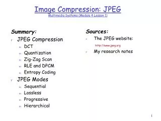
Summary: JPEG Compression DCT Quantization Zig-Zag Scan RLE and DPCM Entropy Coding JPEG Modes Sequential Lossless Progressive Hierarchical. Sources: The JPEG website: http://www.jpeg.org My research notes. Image Compression: JPEG Multimedia Systems (Module 4 Lesson 1). Why JPEG.

E N D
Summary: JPEG Compression DCT Quantization Zig-Zag Scan RLE and DPCM Entropy Coding JPEG Modes Sequential Lossless Progressive Hierarchical Sources: The JPEG website: http://www.jpeg.org My research notes Image Compression: JPEG Multimedia Systems (Module 4 Lesson 1)
Why JPEG • The compression ratio of lossless methods (e.g., Huffman, Arithmetic, LZW) is not high enough for image and video compression. • JPEG uses transform coding, it is largely based on the following observations: • Observation 1: A large majority of useful image contents change relatively slowly across images, i.e., it is unusual for intensity values to alter up and down several times in a small area, for example, within an 8 x 8 image block. A translation of this fact into the spatial frequency domain, implies, generally, lower spatial frequency components contain more information than the high frequency components which often correspond to less useful details and noises. • Observation 2: Experiments suggest that humans are more immune to loss of higher spatial frequency components than loss of lower frequency components.
Fq(u, v) F(u, v) f(i, j) DCT Quantization 8 x 8 8 x 8 JPEG Coding Cr Steps Involved: Discrete Cosine Transform of each 8x8 pixel arrayf(x,y) T F(u,v) Quantization using a table or using a constant Zig-Zag scan to exploit redundancy Differential Pulse Code Modulation(DPCM) on the DC component and Run length Coding of the AC components Entropy coding (Huffman) of the final output Cb Y Quant… Tables Coding Tables Zig Zag Scan Header Tables Data Entropy Coding DPCM RLC
DCT : Discrete Cosine Transform DCT converts the information contained in a block(8x8) of pixels from spatial domain to the frequency domain. • A simple analogy: Consider a unsorted list of 12 numbers between 0 and 3 -> (2, 3, 1, 2, 2, 0, 1, 1, 0, 1, 0, 0). Consider a transformation of the list involving two steps (1.) sort the list (2.) Count the frequency of occurrence of each of the numbers ->(4,4,3,1 ). : Through this transformation we lost the spatial information but captured the frequency information. • There are other transformations which retain the spatial information. E.g., Fourier transform, DCT etc. Therefore allowing us to move back and forth between spatial and frequency domains. 1-D DCT: 1-D Inverese DCT:
Example and Comparison FFT DCT Inverse DCT Inverse FFT Example Description: • f(n) is given from n = 0 to 7; (N=8) • Using DCT(FFT) we compute F(ω) for ω = 0 to 7 • We truncate and use Inverse Transform to compute f’(n)
2-D DCT • Images are two-dimensional; How do you perform 2-D DCT? • Two series of 1-D transforms result in a 2-D transform as demonstrated in the figure below 1-D Column- wise 1-D Row- wise 8x8 8x8 8x8 • F(0,0) is called the DC component and the rest of F(i,j) are called AC components
2-D Transform Example • The following example will demonstrate the idea behind a 2-D transform by using our own cooked up transform: The transform computes a running cumulative sum. 1 1 1 1 1 1 1 1 My Transform: 1 1 1 1 1 1 1 1 1 1 1 1 1 1 1 1 1 1 1 1 1 1 1 1 1 1 1 1 1 1 1 1 8 7 6 5 4 3 2 1 1 1 1 1 1 1 1 1 8 7 6 5 4 3 2 1 1 1 1 1 1 1 1 1 8 7 6 5 4 3 2 1 1 1 1 1 1 1 1 1 1-D Row- wise 8 7 6 5 4 3 2 1 8x8 8 7 6 5 4 3 2 1 64 56 48 40 32 24 16 8 8 7 6 5 4 3 2 1 56 49 42 35 28 21 14 7 8 7 6 5 4 3 2 1 1-D Column- wise 48 42 36 30 24 18 12 6 8 7 6 5 4 3 2 1 40 35 30 25 20 15 10 5 8x8 32 28 24 20 16 12 8 4 24 21 18 15 12 9 6 3 16 14 12 10 8 6 4 2 Note that this is only a hypothetical transform. Do not confuse this with DCT 8 7 6 5 4 3 2 1 8x8
Quantization • Why? -- To reduce number of bits per sample F’(u,v) = round(F(u,v)/q(u,v)) • Example: 101101 = 45 (6 bits). Truncate to 4 bits: 1011 = 11. (Compare 11 x 4 =44 against 45) Truncate to 3 bits: 101 = 5. (Compare 8 x 5 =40 against 45) Note, that the more bits we truncate the more precision we lose • Quantization error is the main source of the Lossy Compression. • Uniform Quantization: • q(u,v) is a constant. • Non-uniform Quantization -- Quantization Tables • Eye is most sensitive to low frequencies (upper left corner in frequency matrix), less sensitive to high frequencies (lower right corner) • Custom quantization tables can be put in image/scan header. • JPEG Standard defines two default quantization tables, one each for luminance and chrominance.
Zig-Zag Scan • Why? -- to group low frequency coefficients in top of vector and high frequency coefficients at the bottom • Maps 8 x 8 matrix to a 1 x 64 vector 8x8 . . . 1x64
DPCM on DC Components • The DC component value in each 8x8 block is large and varies across blocks, but is often close to that in the previous block. • Differential Pulse Code Modulation (DPCM): Encode the difference between the current and previous 8x8 block. Remember, smaller number -> fewer bits 45 45 1x64 1x64 54 9 1x64 1x64 48 -6 1x64 1x64 . . . . . . 32 12 1x64 1x64 36 4 1x64 1x64
RLE on AC Components • The 1x64 vectors have a lot of zeros in them, more so towards the end of the vector. • Higher up entries in the vector capture higher frequency (DCT) components which tend to be capture less of the content. • Could have been as a result of using a quantization table • Encode a series of 0s as a (skip,value) pair, where skip is the number of zeros and value is the next non-zero component. • Send (0,0) as end-of-block sentinel value. . . . . . . 0 0 0 0 0 1 1 0 0 0 0 0 0 0 0 2 1x64 5,1 7,2
Entropy Coding: DC Components • DC components are differentially coded as (SIZE,Value) • The code for a Value is derived from the following table Size_and_Value Table
Entropy Coding: DC Components (Contd..) • DC components are differentially coded as (SIZE,Value) • The code for a SIZE is derived from the following table Example: If a DC component is 40 and the previous DC component is 48. The difference is -8. Therefore it is coded as: 1010111 0111: The value for representing –8 (see Size_and_Value table) 101: The size from the same table reads 4. The corresponding code from the table at left is 101. Huffman Table for DC component SIZE field
Entropy Coding: AC Components • AC components (range –1023..1023) are coded as (S1,S2 pairs): • S1: (RunLength/SIZE) • RunLength: The length of the consecutive zero values [0..15] • SIZE: The number of bits needed to code the next nonzero AC component’s value. [0-A] • (0,0) is the End_Of_Block for the 8x8 block. • S1 is Huffman coded (see AC code table below) • S2: (Value) • Value: Is the value of the AC component.(refer to size_and_value table) Partial Huffman Table for AC Run/Size Pairs
Entropy Coding: Example Example: Consider encoding the AC components by arranging them in a zig-zag order -> 12,10, 1, -7 2 0s, -4, 56 zeros 12: read as zero 0s,12: (0/4)12 10111100 1011: The code for (0/4 from AC code table) 1100: The code for 12 from the Size_and_Value table. 10: (0/4)10 10111010 1: (0/1)1 001 -7: (0/3)-7 100000 2 0s, -4: (2/3)-4 1111110111011 1111110111: The 10-bit code for 2/3 011: representation of –4 from Size_and_Value table. 56 0s: (0,0) 1010 (Rest of the components are zeros therefore we simply put the EOB to signify this fact) 40 12 0 0 0 0 0 0 10 -7 -4 0 0 0 0 0 1 0 0 0 0 0 0 0 0 0 0 0 0 0 0 0 0 0 0 0 0 0 0 0 0 0 0 0 0 0 0 0 0 0 0 0 0 0 0 0 0 0 0 0 0 0 0 0
JPEG Modes Sequential Mode: • Each image is encoded in a single left-to-right, top-to-bottom scan. • The technique we have been discussing so far is an example of such a mode, also referred to as the Baseline Sequential Mode. • It supports only 8-bit images as opposed to 12-bit images as described before.
JPEG Modes Lossless Mode: • Truly lossless • It is a predictive coding mechanism as opposed to the baseline mechanism which is based on DCT and quantization(the source of the loss). • Here is the simple block diagram of the technique: Predictive Difference Huffman EnCoder Lossless Coding
Lossless Mode (Contd..) Predictive Difference: • For each pixel a predictor (one of 7 possible) is used that best predicts the value contained in the pixel as a combination of up to 3 neighboring pixels. • The difference between the predicted value and the actual value (X)contained in the pixel is used as the predictive difference to represent the pixel. • The predictor along with the predictive difference are encoded as the pixel’s content. • The series of pixel values are encoded using huffman coding Notes: • The very first pixel in location (0, 0) will always use itself. • Pixels at the first row always use P1, • Pixels at the first column always use P2. • The best (of the 7) predictions is always chosen for any pixel. C B A X
JPEG Modes Progressive Mode: It allows a coarse version of an image to be transmitted at a low rate, which is then progressively improved over subsequent transmissions. • Spectral Selection : Send DC component and first few AC coefficients first, then gradually some more ACs. Spectral Selection: First Scan: Second Scan: Third Scan: . . Nth Scan: Image Pixels
Progressive Mode • Successive Approximation : All the DCT components are sent few bits at a time: For example, send n1 (say,4) bits (starting with MSB) of all pixels in the first scan, the next n2(say 1) bits of all pixels in the second and so on. Pixels ordered (zig-zag-wise) LSB MSB 7 6 5 4 3 2 1 0 . . . One Pixel First Scan: . . . Second Scan: . . . Third Scan: . . . . . . . 5th Scan:
2x2 2x2 2x2 4x4 Hierarchical Mode • Used primarily to support multiple resolutions of the same image which can be chosen from depending on the target’s capabilities. • The figure here shows a description of how a 3-level hierarchical encoder/decoder works: L4 I4 4x4 Encode I’4 Decode Decode 2x2 - L2 I2 + 2x2 Decode Encode + I’2 Decode + + L1 - I + I’ + Encode Decode Decoding Encoding