Download
1 / 23
230 likes | 260 Views
Learn about time-dependent Schrödinger equation and its practical applications in wave, diffusion, Laplace, and Poisson equations. Explore examples with boundary conditions and superposition of energy eigenstates.

E N D
Lecture 15Solving the time dependent Schrödinger equation • Only 7 lectures left • Read through your notes in conjunction with lecture presentations • Try some examples from tutorial questions or Phils Problems • Email me or come to E47 if anything is unclear • Come to see me before the end of term • Email me over Christmas Remember Phils Problems and your notes = everything http://www.hep.shef.ac.uk/Phil/PHY226.htm
Introduction to PDEs In many physical situations we encounter quantities which depend on two or more variables, for example the displacement of a string varies with space and time: y(x, t). Handing such functions mathematically involves partial differentiation and partial differential equations (PDEs). Wave equation Elastic waves, sound waves, electromagnetic waves, etc. Schrödinger’s equation Quantum mechanics Diffusion equation Heat flow, chemical diffusion, etc. Laplace’s equation Electromagnetism, gravitation, hydrodynamics, heat flow. Poisson’s equation As (4) in regions containing mass, charge, sources of heat, etc.
Introduction to PDEs A wave equation is an example of a partial differential equation You all know from last year that a possible solution to the above is and that this can be demonstrated by substituting this into the wave equation If you make either x or t constant, then you return to the expected SHM case Think of a photo of waves (i.e. time is fixed) y x Or a movie of the sea in which you focus on a specific spot (i.e. x is fixed) y t
Introduction to PDEs Unstable equilibrium Step 1: Let the trial solution be So and Step 2: The auxiliary is then and so roots are Step 3: General solution for real roots is Step 4: Boundary conditions could then be applied to find A and B Thing to notice is that x(t) only tends towards x=0 in one direction of t, increasing exponentially in the other
Introduction to PDEs Harmonic oscillator Step 1: Let the trial solution be So and Step 2: The auxiliary is then and so roots are Step 3: General solution for complex is where a= 0 and b= w so Step 4: Boundary conditions could then be applied to find C and D Thing to notice is that x(t) passes through the equilibrium position (x=0) more than once !!!!
Introduction to PDEs Half-range Fourier sine series where A guitarist plucks a string of length d such that it is displaced from the equilibrium position as shown. This shape can then be represented by the half range sine (or cosine) series.
The One-Dimensional Wave Equation A guitarist plucks a string of length L such that it is displaced from the equilibrium position as shown at t = 0 and then released. Find the solution to the wave equation to predict the displacement of the guitar string at any later time t Let’s go thorugh the steps to solve the PDE for our specific case …..
SUMMARY of the procedure used to solve PDEs 1. We have an equation with supplied boundary conditions 2. We look for a solution of the form 3. We find that the variables ‘separate’ 4. We use the boundary conditions to deduce the polarity of N. e.g. 5. We use the boundary conditions further to find allowed values of k and hence X(x). so 6. We find the corresponding solution of the equation for T(t). 7. We hence write down the special solutions. • By the principle of superposition, the general solution is the sum of all special • solutions.. www.falstad.com/mathphysics.html 9. The Fourier series can be used to find the particular solution at all times.
Solving the time dependent Schrödinger equation The TDSE is a linear equation, so any superposition of solutions is also a solution. For example, consider two different energy eigenstates, with energies E1 and E2. Their complete normalised wavefunctions at t = 0 are: But any superposition such as also satisfies the TDSE, and thus represents a possible state of the system. Recall that all wavefunctions must obey the normalization condition: When we superpose, the resulting wavefunction is no longer normalised. However it can be shown that the normalisation condition is fulfilled so long as:
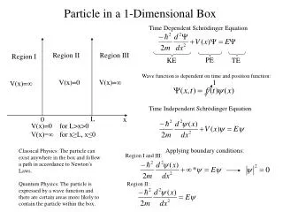
Solving the time dependent Schrödinger equation Consider the time dependent Schrödinger equation in 1 dimensional space: Within a quantum well in a region of zero potential, V(x,t) = 0, this simplifies to: Question Let’s solve the TDSE subject to boundary conditions Y(0, t) = Y(L, t) = 0 (as for the infinite potential well) For all real values of time t and for the condition that the particle exists in a superposition of eigenstates given below at t = 0 .
Solving the time dependent Schrödinger equation n = 1 What does the wavefunction look like? These curves arent normalised – figs intended just to show shape n = 2 Superposition at t = 0 n = 3 If we measure the energy of the state Ψ(x,t) described above we will measure either E1 or E2 or E3 each with the probability of 1/3.
Solving the time dependent Schrödinger equation In a region of zero potential, V(x,t) = 0, so : Step 1: Separation of the Variables Our boundary conditions are true at special values of x, for all values of time, so we look for solutions of the form Y(x, t) = X(x)T(t). Substitute this into the Schrödinger equation: Step 2: Rearrange the equation Separating variables:
Solving the time dependent Schrödinger equation Step 3: Equate to a constant Now we have separated the variables. The above equation can only be true for all x, t if both sides are equal to a constant. It is conventional (see PHY202!) to call the constant E. So we have: which rearranges to (i) (ii) which rearranges to
Solving the time dependent Schrödinger equation Step 4: Decide based on situation if E is positive or negative We have ordinary differential equations for X(x) and T(t) which we can solve but the polarity of E affects the solution ….. For X(x) Our boundary conditions are Y(0, t) = Y(L, t) = 0, which means X(0) = X(L) = 0. So clearly we need E > 0, so that equation (i) has the form of the harmonic oscillator equation. It is simpler to write (i) as: where giving
Solving the time dependent Schrödinger equation Step 5: Solve for the boundary conditions for X(x) For X(x) Our boundary conditions are Y(0, t) = Y(L, t) = 0, which means X(0) = X(L) = 0. If where then applying boundary conditions gives X(0) = 0 gives A = 0 ; we must have B ≠ 0 so X(L) = 0 requires , i.e. so for n = 1, 2, 3, ….
Solving the time dependent Schrödinger equation Step 6: Solve for the boundary conditions for T(t) A couple of slides back we decided that in order to have LHO style solutions for X(x) we must have E > 0. So here we must also take E > 0. Equation (ii) has solution as it’s only a 1st order ODE Proof of statement above Replace the constant with T0
Solving the time dependent Schrödinger equation Step 7: Write down the special solution for Y (x, t) where (These are the energy eigenvalues of the system.) Question asks for the solutions of the TDSE for real values of time where Real values are therefore
Solving the time dependent Schrödinger equation Step 8: Constructing the general solution for Y (x, t) We have special solutions: The general solution of our equation is the sum of all special solutions: (In general therefore a particle will be in a superposition of eigenstates.)
Solving the time dependent Schrödinger equation Step 10: Finding the full solution for all times The general solution is If we know the state of the system at t = 0, we can find the state at any later time. Since we said that At t = 0 the general solution is Then we can say: where and Superposition at t = 0
Particular solution to the time dependent Schrödinger equation Y3 Y2 1st Eigenfunction Y1 3rd Eigenfunction 2nd Eigenvalue 3rd Eigenvalue 1st Eigenvalue
Solving the time dependent Schrödinger equation where Superposition at t = 0 and In this particular example Ψ(x,t) is composed of eigenstates with different parity (even and odd). Therefore Ψ(x,t) does not have a definite parity and P(x,t) oscillates from side to side. www.falstad.com/mathphysics.html • 1. Energy eigenstates (namely, states with definite energy) are stationary states: they have constant probability densities and definite energies. • 2. Mixed states (namely, superpositions of energy eigenstates) do not have a definite energy but have a probability of being in any one of the energy states when measured. • 3. The probability densities of mixed states vary with time as do therefore the < x >.
Just for Quantum Mechanics course The expectation value is interpreted as the average value of x that we would expect to obtain from a large number of measurements. NB. In order to have time dependence in any observable such as position, it is necessary for the wavefunction to contain a superposition of states with different energies. This is because the probability density for a mixed state varies with time, whereas for a pure state it is constant in time. Pure states are known as stationary states. For example if we have the single eigenfunction within an infinite potential well then and . Notice how there is no time dependence. www.falstad.com/mathphysics.html This means < x > is invariant with time
Just for Quantum Mechanics course But if we add another eigenfunction for example: The complex conjugate is written as: Therefore: Let eigenfunctions be: So: A superposition of eigenstates having different energies is required in order to have a time dependence in the probability density and therefore in < x >. Non zero so long as E1≠ E2