091 h s
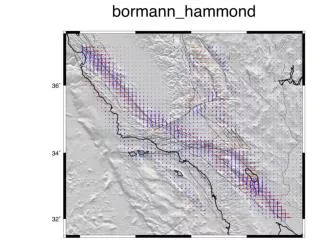
091 h s. Jayne Bormann and Bill Hammond sent two velocity fields on a uniform grid constructed from their test exercise using CMM4. Hammond ’ s code was used. Surface creep was not included and a uniform locking depth of 15 km was used. 095 h s.

091 h s
E N D
Presentation Transcript
091 hs Jayne Bormann and Bill Hammond sent two velocity fields on a uniform grid constructed from their test exercise using CMM4. Hammond’s code was used. Surface creep was not included and a uniform locking depth of 15 km was used.
095 hs The GPS data for the western US are obtained from PBO velocity at UNAVCO site, Southern California Earthquake Center California Crustal Motion Map 1.0, McCaffrey et al. (2007) for Pacific Northwest, the GPS velocity field of Nevada and its surrounding area from the Nevada Geodetic Lab at the University of Nevada at Reno, and the GPS velocity field of the Wasatch-Front and the Yellowstone-Snake-River-River-Plain network from Bob Smith of University of Utah. These separate velocity fields are combined by adjusting their reference frames to make velocities match at collocated stations. I determined the Voronoi cells for this combined GPS stations and used their areas to weight the corresponding stations for inversion. I then interpolated those GPS observation into uniform grid point for the western US using the method of Wald (1998) and calculated the final strain rate map. A' B' A C' B C
111 hs What I do is use an anisotropic variance-covariance matrix for the strain rates. I do not build in fault slip rates, but I use the variance-covariance matrix to place a priori constraints on expected shear directions as well as some constraints on expected shear magntitudes. However, in the end the GPS velocities dictate the actual strain rates and styles of strain rate (where they are high, low, etc.). I am also limited by the finite-element grid, which is .1x.1 degree grid area spacing. It might be worthwhile to compare the solution I sent you with one obtained using fully isotropic uniform variances for all areas. That is, with an a priori expected strain rate distribution that is everywhere uniform. I can look into the reduced chi-squared misfit for both of these cases.
123 hs Strain rate derived from a dislocation model of the San Andreas Fault system [Smith-Konter and Sandwell, GRL, 2009]. 610 GPS velocity vectors were used to develop the model. The model consists of an elastic plate over a visco-elastic half space at 1 km horizontal resolution. Deep slip occurs on 41 major fault segments where rate is largely derived from geological studies. The locking depth is varied along each fault segment to provide a best fit to the GPS data. The model is fully 3-D and the vertical component of the GPS vectors is also used in the adjustment. An additional velocity model was developed by gridding the residuals to the GPS data using the GMT surface program with a tension of 0.35. This was added to the dislocation model.
147 hs The strains are calculated analytically using elastic dislocation theory in a homogeneous elastic halfspace. The model is subset of a western US block model geodetically constrained by a combination of the SCEC CMM 3.0, McClusky ECSZ, Hammond Walker Lane, McCaffrey PNW, d'Allessio Bay Area, and PBO velocity fields. These are combined by minimizing residuals (6-parameter) at collocated stations. In southern California the block geometry is based on and the Plesch et al., CFM-R and features dipping faults in the greater Los Angeles regions which end up producing some intricate strain rate patterns. The model features fully coupled (locked from the surface to some locking depth) faults everywhere except for Parkfield, the SAF just north, and the Cascadia subduction zone. For Parkfield and Cascadia we solve for smoothly varying slip on surfaces parameterized using triangular dislocation elements.
114 hs Strain rate tensor model derived from fitting a continuous horizontal velocity field through GPS velocities [Kreemer et al, 2009]. 2053 GPS velocities were used, of which 854 from our own analysis of (semi-)continuous sites and 1199 from published campaign measurements (all transformed into the same reference frame). The model assumes that the deformation is accommodated continuously, and lateral variation in damping is applied to ensure that the reduced chi^2 fit between observed and modeled velocities is ~1.0 for subregions.