Transportation Model
Transportation Model. Basic Problem

Transportation Model
E N D
Presentation Transcript
Basic Problem The basic idea in a transportation problem is that there are sites or sources of product that need to be shipped to destinations. Typically the routes and the amounts shipped on each route must be determined and the goal is to minimize the cost of shipping. The constraints are that you can not ship more from a source than made at that source and you do not want to ship more to a place than needed. Some vocabulary: Source or origin is supply. Factory capacity is supply. Destination is demand. Warehouse requirements can also be called demand. (Supply and demand here are not exactly as would be used in an economics class.)
Some assumptions If production costs are the same at each source, ignore them. If they are not the same include them in the analysis. From a given site to a given destination, shipping costs per unit are the same no matter the volume of shipping. We have a balanced problem, or the total amount from sources add up to the total demand at destinations – we change this later.
Let’s do an example to highlight details of the work needed to arrive at the optimal solution. Say the following amounts are made at the various sources: Des Moines 100 (units) Evansville 300 Ft. Lauderdale 300 and say the following sites demand the amounts shown, Albuquerque 300 Boston 200 Cleveland 200 (note the balance of supply and demand).
Say the costs of shipping a unit from each source to each destination is as in the following table:
In this problem we have three origins of product. In general we will use the index i to represent origin i. Here i goes from 1 to 3. Lets make Des Moines = 1, Evansville = 2 and Ft. Lauderdale = 3. We use the index j to represent destinations. Here j also goes from 1 to 3 and let’s make Albuquerque = 1, Boston = 2 and Cleveland = 3. Xij = the amount shipped from source or origin i to destination j. The objective in a transportation problem is to minimize the cost of shipping. In our problem the objective is Min 5X11 + 4X12 + 3X13 + 8X21 + 4X22 + 3X23 + 9X31 + 7X32 + 5X33 Note that in the objective function I put the first origin, Des Moines, first to each of the destinations. Then do all from Evansville, and so on. The coefficients on the X’s are the shipping costs.
Now each origin and each destination will contribute 1 constraint each on the problem. For example, Des Moines as an origin can only ship as much as 100 units. Since there are three destinations here the Des Moines constraint is X11 + X12 + X13 ≤ 100. This means the amount shipped in total to the three destinations can not exceed 100 units. Note the first subscript on the X’s is 1 for Des Moines and note the coefficients on the X’s are all 1. Similarly for Evansville and Ft. Lauderdale we have, respectively, X21 + X22 + X23 ≤ 300, and X31 + X32 + X33 ≤ 300. Now, on the demand side we assume if a destination has a demand it needs to get that amount so we make the constraints equalities. Note, when I have the demand constraints on the next page, the second subscript will be the same in a given constraint because the destination is the 1 site.
Demand Constraints Albuquerque X11 + X21 + X31 = 300 (the amount from each source to Albuquerque must add in total to 300.) Boston X12 + X22 + X32 = 200, and Cleveland X13 + X23 + X33 = 200 The Management Scientist Linear Programming software can be used to solve the problem. On the next slide I put all the constraints and the objective function together.
Min 5X11 + 4X12 + 3X13 + 8X21 + 4X22 + 3X23 + 9X31 + 7X32 + 5X33 s.t. X11 + X12 + X13 ≤ 100 X21 + X22 + X23 ≤ 300 X31 + X32 + X33 ≤ 300 X11 + X21 + X31 = 300 X12 + X22 + X32 = 200 X13 + X23 + X33 = 200 I spread the constraints out to get you to visualize what the input will look like in the software. When you see a space leave a blank. Your input will look like X11 X12 X13 X21 X22 X23 X31 X32 X33 5 4 3 8 4 3 9 7 53 1 1 1 ≤ 100 1 1 1 ≤ 300 1 1 1 ≤ 300 1 1 1 = 300 1 1 1 = 200 1 1 1 = 200 The output from the program is on the 2 next slides (I had to take it in 2 parts.)
This is the minimum cost Ship on x11, which is Des Moines to Al. – and so on Note there is no shipping from Des Moines to Boston in the optimal solution. The reduced cost on this has the interpretation that if you shipped a unit on this route cost would go up by 2.
The first three constraints are for the origins. These Dual Price numbers mean how much cost would fall if you had one more unit supply from the appropriate origin. The upper limits on the demand constraints are reached. The dual prices for these constraints are negative. They represent what would happen to cost if demand fell 1 unit. So if 4th constraint became 299 cost would be 3900-9 = 3891.
Now, there is a different module in the software that will do transportation problems. But, it just tells how much to ship on which routes. You do not get the sensitivity analysis that we just went through in linear programming. The input is way easier though. If you are in the linear programming module you can go to file and scroll to change modules. Then you would check Transportation and hit OK. Then you would go to file, new. At the next screen type in the number of origins and the number of destinations and hit ok. Then your input screen would look like what is on the next screen. You would type in the numbers.
When you type the data in and go to solve you have to tell whether you have a max problem or a min problem. This was a min. Here we have the results. You get the low cost and which routes to ship on. This method has easy set up and easy answer – no sensitivity analysis – but who needs sensitivity analysis anyway !