From-Point Occlusion Culling
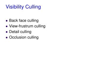
From-Point Occlusion Culling. Chapter 23. Talk Outline . Image space methods Hierarchical Z-Buffer Hierarchical occlusion maps Some other methods Object space methods General methods Shadow frusta, BSP trees, temporal coherent visibility Cells and portals.


From-Point Occlusion Culling
E N D
Presentation Transcript
From-Point Occlusion Culling Chapter 23
Talk Outline • Image space methods • Hierarchical Z-Buffer • Hierarchical occlusion maps • Some other methods • Object space methods • General methods • Shadow frusta, BSP trees, temporal coherent visibility • Cells and portals
What Methods are Called Image-Space? • Those where the decision to cull or render is done after projection (in image space) Decision to cull Object space hierarchy View volume
Ingredients of an Image Space Method • An object space data structure that allows fast queries to the complex geometry Regular grid Space partitioning Hierarchical bounding volumes
An Image Space Representation of the Occlusion Information • Discrete • Z-hierarchy • Occlusion map hierarchy • Continuous • BSP tree • Image space extends
General Outline of Image Space Methods • During the in-order traversal of the scene hierarchy do: • compare each node against the view volume • if not culled, test node for occlusion • if still not culled, render objects/occluders augmenting the image space occlusion • Most often done in 2 passes • render occluders – create occlusion structure • traverse hierarchy and classify/render
Testing a Node for Occlusion • If the box representing a node is not visible then nothing in it is either • The faces of the box are projected onto the image plane and tested for occlusion occluder hierarchical representation
Testing a Node for Occlusion • If the box representing a node is not visible then nothing in it is either • The faces of the box are projected onto the image plane and tested for occlusion occluder hierarchical representation
Differences of Algorithms • The most important differences between the various approaches are: • the representation of the (augmented) occlusion in image space and, • the method of testing the hierarchy for occlusion
Hierarchical Z-Buffer (HZB) (Greene and Kass, SIG 93) • An extension of the Z-buffer VSD algorithm • It follows the outline described above • Scene is arranged into an octree which is traversed top-to-bottom and front-to-back • During rendering the Z-pyramid (the occlusion representation) is incrementally built • Octree nodes are compared against the Z-pyramid for occlusion
The Z-Pyramid • The content of the Z-buffer is the finest level in the pyramid • Coarser levels are created by grouping together four neighbouring pixels and keeping the largest z-value • The coarsest level is just one value corresponding to overall max z
The Z-Pyramid = furthest Objects are rendered = closer = closest Depth taken from the z-buffer Construct pyramid by taking max of each 4
Using The Z-Pyramid = furthest = closer = closest
Maintaining the Z-Pyramid • Ideally every time an object is rendered causing a change in the Z-buffer, this change is propagated through the pyramid • However this is not a practical approach
More Realistic Implementation • Make use of frame to frame coherence • at start of each frame render the nodes that were visible in previous frame • read the z-buffer and construct the z-pyramid • now traverse the octree using the z-pyramid for occlusion but without updating it
HZB: Discussion • It provides good acceleration in very dense scenes • Getting the necessary information from the Z-buffer is costly • A hardware modification was proposed for making it real-time
Hierarchical Occlusion Maps (Zhang et al, SIG 97) • Similar idea to HZB but • they separate the coverage information from the depth information, two data structures • hierarchical occlusion maps • depth (several proposals for this) • Two passes • render occluders and build HOM • render scene hierarchy using HOM to cull
What is the Occlusion Map Pyramid? • A hierarchy of occlusion maps (HOM) • At the finest level it’s just a bit map with • 1 where it is transparent and • 0 where it is opaque (ie occluded) • Higher levels are half the size in each dimension and store gray-scale values • Records average opacities for blocks of pixels • Represents occlusion at multiple resolutions
Occlusion Map Pyramid 64 x 64 32 x 32 16 x 16
How is the HOM Computed? • Clear the buffer to black • Render the occluders in pure white (no lighting, textures etc) • The contents of the buffer form the finest level of the HOM • Higher levels are created by recursive averaging (low-pass filtering) • Construction accelerated by hardware - bilinear interpolation or texture maps / mipmaps
Overlap Tests • To test if the projection of a polygon is occluded • find the finest-level of the pyramid whose pixel covers the image-space box of the polygon • if fully covered then continue with depth test • else descend down the pyramid until a decision can be made
Transformed view-frustum D. E. B. Image plane Bounding rectangle at farthest depth Image plane The plane Bounding rectangle at nearest depth Occluders The point with nearest depth Viewing direction B Viewing direction Occluders A This object passes the depth test A Resolving Depth Either: a single plane at furthest point of occluders Or: uniform subdivision of image with separate depth at each partition Or even: just the Z-buffer content
1 0 2 3 4 Aggressive Approximate Culling
HP Hardware implementation • Before rendering an object, scan-convert its bounding box • Special purpose hardware are used to determine if any of the covered pixels passed the z-test • If not the object is occluded
Read top half of the buffer to use as an occlusion map Project top of cell to image space Simplify projection to a line Test if any pixel along line is visible Simplified Occlusion Map
Discussion on Image Space • Advantages (not for all methods) • hardware acceleration • generality (anything that can be rendered can be used as an occluder) • robustness, ease of programming • option of approximate culling • Disadvantages • hardware requirements • overheads
Object Space Methods • Visibility culling with large occluders • Hudson et al, SoCG 97 • Bittner et al, CGI 98 • Coorg and Teller, SoCG 96 and I3D 97 • Cells and portals • Teller and Sequin, Siggraph 91 • Luebke and Georges, I3D 95
Occlusion Using Shadow Frusta(Hudson et al, SoCG 97) Occluder A Viewpoint B C
Assuming we can Find Good Occluders • For each frame • form shadow volumes from likely occluders • do view-volume cull and shadow-volume occlusion test in one pass across the spatial sub-division of the scene • each cell of the sub-division is tested for inclusion in view-volume and non-inclusion in each shadow volume
Occluder Test • Traverse the scene hierarchy top down • Overlap test (cell to shadow volume) is performed in 2D • when the hierarchy uses an axis-aligned scheme (eg kd-trees, bounding boxes etc) then a very efficient overlap test is presented
Occlusion Trees (Bittner et al, CGI 98) • Just as before • scene represented by a hierarchy (kd-tree) • for each viewpoint • select a set of potential occluders • compare the scene hierarchy for occlusion • However, unlike the previous method • the occlusion is accumulated into a binary tree • the scene hierarchy is compared for occlusion against the tree
Create shadow volume of occluder 1 out out out IN O3 Tree 1 O2 2 View point O1 2 O1 1
Insert occluder 2 and augment tree with its shadow volume out out out out IN IN O3 Tree 4 1 O2 2 View point O1 3 3 2 out O1 4 1 O2
And so on until all occluders are added out out out out out out 3 IN IN IN 4 O2 O3 Tree 4 1 O2 O4 2 View point O1 3 2 out O1 5 1 6 O3
Check occlusion of objects T1 and T2 by inserting them in tree out out out out out out 3 IN IN IN 4 O2 O3 Tree 4 1 O2 2 View point O1 3 2 out O1 T2 5 1 6 O3 T1
Occluder selection • This is a big issue relevant to most occlusion culling algorithms but particularly to the last two • At pre-processing • Identify likely occluders for a cell • they subtend a large solid-angle • Test likely occluders • use a sample of viewpoints and compute actual shadow volumes resulting • At run time • locate the viewpoint in the hierarchy and use the occluders associated with that node
Metric for Comparing Occluder Quality Occluder quality: (-A *(N • V)) / ||D||2 A : the occluder’s area N : normal V : viewing direction D : the distance between the viewpoint and the occluder center
Cells and Portals(Teller and Sequin, SIG 91) • Decompose space into convex cells • For each cell, identify its boundary edges into two sets: opaque or portal • Precompute visibility among cells • During viewing (eg, walkthrough phase), use the precomputed potentially visible polygon set (PVS) of each cell to speed-up rendering
S•L 0, L L S•R 0, R R Find_Visible_Cells(cell C, portal sequence P, visible cell set V) V=V C for each neighbor N of C for each portal p connecting C and N orient p from C to N P’ = P concatenate p if Stabbing_Line(P’) exists then Find_Visible_Cells (N, P’, V) Compute Cell Visible From EachCell Linear programming problem:
Eye-to-Cell Visibility • A cell is visible if • cell is in VV • all cells along stab tree are in VV • all portals along stab tree are in VV • sightline within VV exists through portals • The eye-to-cell visibility of any observer is a subset of the cell-to-cell visibility for the cell containing the observer
Instead of pre-processing all the PVS calculation, it is possible to use image-space portals to make the computation easier Can be used in a dynamic setting Image Space Cells and Portals (Luebke and Georges, I3D 95)
Discussion on Object Space • Visibility culling with large occluders • good for outdoor urban scenes where occluders are large and depth complexity can be very high • not good for general scenes with small occluders • Cells and portals • gives excellent results IF you can find the cells and portals • good for interior scenes • identifying cells and portals is often done by hand • General polygons models “leak”
Conclusion • There is a very large number of point-visibility algorithms • Image space are becoming more and more attractive • Specialised algorithms should be preferred if speed is most important factor