Download
1 / 33
330 likes | 345 Views
Property Rights and Collective Action in Natural Resources with Application to Mexico. Lecture 1: Introduction to the political economy of natural resources Lecture 2: Theories of collective action, cooperation, and common property

E N D
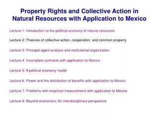
Property Rights and Collective Action in Natural Resources with Application to Mexico Lecture 1: Introduction to the political economy of natural resources Lecture 2: Theories of collective action, cooperation, and common property Lecture 3: Principal-agent analysis and institutional organization Lecture 4: Incomplete contracts with application to Mexico Lecture 5: A political economy model Lecture 6: Power and the distribution of benefits with application to Mexico Lecture 7: Problems with empirical measurement with application to Mexico Lecture 8: Beyond economics: An interdisciplinary perspective
Why property rights important • Allow markets to function • Increase incentives to invest • If transaction costs = 0, fully defining property rights gets us to an efficient outcome
Transaction costs • If transaction costs > 0, asset ownership confers power • Transaction costs of an exchange: • Negotiating the agreement • Writing a contract • Observing/monitoring the agreement • Enforcing agreement of contract is broken
What is a property right? • Residual rights of control • Ability to specify unspecified uses • Ability to alienate others from use of the property • Whoowns what determines efficiency if transaction costs > 0 • Incomplete contract (IC) theory: concerned with the most efficient allocation of property rights.
What is an incomplete contract? • Transaction costs make contracts incomplete • Bounded rationality: • Background assumption to incomplete contracts. • Cannot think through all branches of a decision tree. • Cannot represent everything in a contract. • E.g. complicated bilateral relations. • People deal with this bounded rationality in a substantively rational way.
Incomplete Contract Theory • Grossman and Hart (1986) • Hart and Moore (1990) • Hart (1995) • Different than Williamsonian transaction costs analysis • Allows renegotiation
Model • 2 parties: i = A and B • Each party may be an “expert” to work with some physical asset KA and KB respectively • Both parties A and B can expend investments (a and b, respectively) in human capital • These investments are nonverifiable • Other party cannot buy this capital
Model Notation • Let K = {KA, KB} • Ki is set of asset owned by i • Denote KA KB = K • Denote KA KB =
Default payoffs • Individual payoffs if do NOT work together: VA[KA, a, 0] VA[KA,a] VB[KB, 0, b] VB[KB,b]
Payoffs with Trade • Total payoffs if work together: V[K, a, b] Payoff to us: less notation!
Physical Asset versus Human Capital (or Relationship) Specificity Investment ai party i is: • Nonspecific when the marginal return does not depend on Kj nor aj • Purely relationship specific when the marginal return is 0 unless parties work together • Relationship specific when the marginal return positively depends on access to aj • Purely asset specific if the marginal return depends (only) on party i’s access to Kj
Basic Assumptions • V[K, a, b] > VA[KA,a] + VB[KB,b] Ki GAINS TO TRADE: it is efficient to work together Let ai = {a if i=A, b if i=B} • Vai [.] Viai [K, ai] Viai [Ki, ai] Vai [Kj, ai] Vai [, ai] Marginal returns from investments are weakly larger the more human and physical capital a party has access to, i.e. relationship specificity exists.
Asset complementarity • An asset is complementary when: Viai [K, ai] > Viai [Ki, ai] (access to both assets K makes you more productive) • An asset is strictly complementary when: Viai [Ki, ai] goes to 0 (you need access to Kj as well) • An asset is independent when: Viai [K, ai] = Viai [Ki, ai] (one asset suffices for your productivity)
Equilibrium analysis • Backwards induction: start with Date 2 • Date 2: Investments a and b are “sunk” • Since V(.) > VA (.) + VB(.) a,b,Ki, then parties will agree on “working together” but choose investments noncooperatively ex post efficiency • Division of joint surplus V(.): Nash bargaining solution • Party i obtains: • Default payoff: Vi[Ki ,ai] • Fraction i [0,1] of “excess surplus”: V = V(.) - VA (.) - VB(.)
Who should own what? • Compare investments levels under various ownership configurations and contracting conditions (e.g. specificity, complementarity, cooperative v. noncooperative investments) • The configuration yielding highest total surplus (both A and B’s payoffs combined) is most efficient given the conditions.
A owns KA and KB: Integration UIA = VA[K, a] + A[V[K,a,b] - VA[KA,a] -VB[,b] ] - a UIB = VB[0, b] + (1-A)[V[K,a,b] - VA[KA,a] -VB[,b] ] – b FOCs: A: (1- A) VAa [K, a] + A Va [K, a, b] = 1 aI B: A VBb[,b] + (1- A) Vb [K, a, b] = 1 bI
A owns KA, B owns KB: Nonintegration UNIA = VA[KA, a] + A[V[K,a,b] - VA[KA,a] -VB[KB,b] ] - a UNIB = VB[KB, b] + (1-A)[V[K,a,b] - VA[KA,a] -VB[KB,b] ] – b FOCs: A: (1- A) VAa [KA, a] + A Va [K, a, b] = 1 aNI B: A VBb[KB,b] + (1- A) Vb [K, a, b] = 1 bNI
First-Best Efficient Outcomes • Parties “work together” and choose investments cooperatively first-best outcome • Investment levels are: [a*, b*] = argmaxa,b V{K,a,b] – a – b FOCs: Va = 1 ; Vb = 1 Simple!
First Result • Under any ownership structure (i.e. integration or nonintegration) there is underinvestment in relationship-specific investments (Hart 1995), that is: a* > aI or aNI and b* > bNI or bI
Marginal productivity of investments 1 a* aNI aI
Other Results • If investments by one party are inelastic, then integration by the other party is optimal • If assets are independent, then nonintegration is optimal • If assets are complementary, then some form of integration is desirable. • If one party’s HK is essential, then integration by that party is optimal • If both parties’ HK are essential, then all ownership types are equally optimal.
Critique of Incomplete Contracts • Maskin and Tirole (1999): • Agents have bounded rationality but deal with noncontractibility in a rational way • does BR constrain set of feasible contracting outcomes relative to complete contracts? • Counter-theorem: Nondescribability is irrelevant under certain conditions • Segal and Hart: as number of possible states of world increase, null (incomplete) contract is optimal.
Application to Mexico Community Forestry Production • What explains the vertical integration pattern across Mexican communities with forest? • Apply and extend incomplete contract model • Assume two parties: • A = community • B = downstream firm/buyer • Assets: • Forest land, extraction equipment, milling and processing equipment.
Examples of Unforeseeables • Rainy season • Access problems • Equipment failure • Scheduling problems • Timber condition • Failure to pay, deliver • Un-monitored extraction
An IC Model • Survey data from 43 observations in Oaxaca (see Antinori (2000)) • Ownership possibilities: • Assume communities can own forest land and any downstream equipment • Assume outside private firms can own any downstream equipment for wood production and can contract with communities for raw material. • Tradeoffs: need for specialized expertise and overcoming collective action hurdles v. benefits of ownership (see Antinori and Rausser (2007) for details)
Econometric Model of Vertical Integration • Ordered logit (see paper for details) • Dependent variable: level of community vertical integration (sale of stumpage, roundwood, lumber of secondary goods) • Independent variables: • Influences on ability to coordinate, produce: • Past mechanical training (+ and significant) • Initial logging roads (not significant) • Parastatal existence (+ and significant) • Contracting costs, valuation: • Forested hectares (+ and significant) • Forest quality (initial) (+ and significant) • Distance to pop center (+ and significant) • Non-commercial timber forest uses (not significant)
Conclusions • Ownership of assets critical for control over benefits when transaction costs present • Limitations of PR approach: • Collective decisionmaking still not completely modeled in firm. • Beyond property rights as control over assets
Asset Wealth • Oliver and Shapiro: Black Wealth/White Wealth: • Persistent wealth gap versus income gap in the United States between black and white • Limits opportunities