Download
1 / 15
150 likes | 257 Views
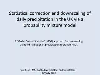
Statistical correction and downscaling of daily precipitation in the UK via a probability mixture model. A ‘Model Output Statistics’ (MOS) approach for downscaling the full distribution of precipitation to station-level. Tom Kent – MSc Applied Meteorology and Climatology 23 rd July 2012.

E N D
Statistical correction and downscaling of daily precipitation in the UK via a probability mixture model A ‘Model Output Statistics’ (MOS) approach for downscaling the full distribution of precipitation to station-level. Tom Kent – MSc Applied Meteorology and Climatology 23rd July 2012
Central aim: • To develop an eventwise GCM-based MOS model for downscaling the full distribution, including extremes, of daily precipitation at point locations (i.e. station level) using nudged GCM-simulated precipitation as the predictor. • 2 Stages: • Stationary model – fitting the mixture model to observations. • Non-stationary model – development of a univariate VGLM mixture model
Development of a univariate mixture model Based on Frigessi et al. (2002), applied in this form by Vrac and Naveau(2007): univariate probability mixture model that merges classical (e.g. Gamma dist., ) and EV distributions (e.g. GPD, ) to model the full distribution, , of precipitation. where Location of transition from Gamma to GPD density Weight function: Non-decreasing; takes values in (0,1] Transition rate • w provides a smooth transition from gamma to GPD density and so the full distribution f is continuous. • Threshold selection is replaced by an unsupervised estimation procedure, namely finding from the data. • Result: • The full distribution of precipitation, including extremes, is modelled via a probability mixture model without threshold selection.
Before downscaling…. Assessing the sensitivity of the mixture model parameters in a stationary setting • Number of years = 44 (years 1958-2001) • Leave one year out of the estimation procedure so that the model’s parameters are estimated from a 43 year subset of the data. • Result: 44 sets of mixture model parameters are estimated from the 44 subsets of the observational data.
Data: Oxford DJF and JJA Daily observed precipitation 1958-2001. Dry threshold: >1mm
A closer look at the behaviour of m (the location of transition between Gamma and GPD) DJF: 90th percentile (from obs.) = 10.9mm 95th percentile = 14.4mm JJA: 90th percentile (from obs.) = 13.2mm 95th percentile = 18.5mm
A closer look at the behaviour of xi: • when xi is positive, the upper tail of the distribution is unbounded • when xi is negative, the upper tail is bounded When xi < 0, is a Gamma distribution alone more appropriate?
QQ Plots: Oxford JJA Gamma distribution Mixture model distribution
QQ Plots: Oxford DJF Gamma distribution Mixture model distribution
The effect of the sensitivity of the parameters on the mixture model pdfs: Histogram: wet (>1mm) precipitation measurements from Oxford. Red lines: mixture model pdfs determined by the different ‘leave-one-out’ subsets
The problem of tau… • In the estimation procedure, tau almost always tends to its pre-set lower bound, i.e. 1e-12. • Consequently: • abrupt change from Gamma to GPD • un-smoothness in the pdf, i.e. a ‘kink’ occurs where . • Possible solution..? • Remove tau from the estimation procedure, i.e. fix it beforehand so that the likelihood function is a function of 5 parameters only. MLE is then performed for a range of fixed tau values… • The behaviour of the remaining 5 parameters can then be analysed for various fixed tau values
Spread/skill of the 5 mixture model parameters as a result of the leave-one-out estimation WITH TAU FIXED beforehand
Key points… • relatively small spread (i.e. high skill) for tau close to zero • relationship between m and tau: as tau decreases, m increases. • For tau close to zero, m≈13; this seems reasonable as location transition between Gamma and GPD. • But small tau implies “unsmoothness”; thus, it seems to be a trade-off between m and tau. Final (??) decision: Fix tau, leave m in the estimation procedure.
Using the model to downscale: a univariate VGLM mixture model Downscaling (and predictive ability) of precipitation is achieved through employing VGLMs to the mixture model parameters . If there are n predictors, x, at each time step i: GPD Gamma distribution Fixed?? Weight function are estimated by fitting the model to observed rainfall.
Thank you for listening… … any questions?