Download
1 / 27
270 likes | 447 Views
Potential and limits of satellite data for climate issues Hans von Storch 12 , Matthias Zahn 12 , Anne Blechschmidt 2 , Stiig Wilkenskjeld 1 , Heinz Günther 1 and Stephan Bakan 23 EXTROP Virtual Institute and 1 Institute for Coastal Research, GKSS Research Center, Germany

E N D
Potential and limits of satellite data for climate issues Hans von Storch12, Matthias Zahn12, Anne Blechschmidt2, Stiig Wilkenskjeld1, Heinz Günther1 and Stephan Bakan23 EXTROP Virtual Institute and 1 Institute for Coastal Research, GKSS Research Center, Germany 2 Meteorological Institute of the University of Hamburg, Germany 3 Max-Planck Institute of Meteorology, Germany
Overview • Satellite products are useful – in some, even many cases • But the utility of satellite products in climate research is limited – by the length of available time series and compromised by their homogeneity • Examples:1) Analysis of polar low occurrence2) Derivation of information about tails of distributions (extreme wave heights) • Results from satellite-climate modeller interaction in the HGF virtual institute EXTROP
Impact of satellite data on forecast skill Anomaly correlation Source: The Changing Earth (SP-1304, ESA, 2006) Increase in anomaly correlation of 500hPa height forecasts during recent decades is to a large extent due to the assimilation of satellite data
Decline in Arctic sea ice extent Source: The Changing Earth (SP-1304, ESA, 2006) Minimum sea ice extent for the month of Sept. each year. Ice extent is defined as area with an ice concentration >15%
Global sea level rise Source: The Changing Earth (SP-1304, ESA, 2006) Sea level rise derived from several satellite altimeters
Climate research deals with (changing) statistics of parameters characterising weather. It deals to large extent with the inference of characteristic parameters such as spatial disaggregated mean values or average occurrences of certain phenomena, extreme values, spatial correlations, spectra and characteristic patterns, and sensitivities. To do proper inference the data need to fulfil some properties. 1. The data must be representative of the considered statistical ensembles, i.e., the time series must be long enough. 2. Second, the data should be homogeneous, i.e., the informational content should be the same through the entire time series.
We examine two examples, which illustrate the potential and limit of using satellite data – the first deals with scrutinizing the skill of a climate model, and the other with the number of samples and accuracy needed to infer extreme value statistics from satellite soundings. PhD work done at the Virtual Institute EXTROP by • Anne Blechschmidt (HOAPS data set) • Matthias Zahn (Polar Low simulations) • Stiig Wilkenskjeld (Simulation of satellite based inference of significant wave height)
1st Case: Polar Lows The task/aim is to determine the occurrence of polar lows in the sub-polar Atlantic in the past decades. Eventually this will enable an assessment whether recent trends in frequency, spatial distribution or intensity are consistent with climate change scenarios or not. In-situ data for this purpose are not available; (passive or active) satellite data are available only for a limited time. On the other hand, downscaling strategies, involving a limited area atmospheric model suitably embedded in global atmospheric re-analysis, are able to generate mesoscale disturbances in climate mode simulations. We demonstrate the quality of the LAM simulation by comparing the model simulation with the HOAPS climatology in a case study, when high-quality satellite data are available.
Two year climatology of polar lows • Study area: Nordic Seas • Visual inspection of AVHRR images • Usage of HOAPS-S wind estimates (> 15 m/s required for meso-scale disturbance to count as polar low) • When no wind estimate is available, cases are classified as “PL-like” • Problem: only two years of data screened (very work-intensive) Anne Blechschmidt
Key features of HOAPS 3Hamburg OceanAtmosphereParameters and Fluxes fromSatellite Data precipitation, evaporation and related sea surface and atmospheric state parameters over ice-free oceans derived from the SSM/I (passive microwave) radiometer on board the polar orbiting DMSP satellites precipitation, surface wind speed and near surface air humidity (among others) directly retrieved evaporation is derived through a bulk transfer formula, for which the additionally necessary sea surface specific humidity is calculated from the NOAA Pathfinder SST, which uses AVHRR data 18+ years of satellite data: 1987 – 2005 homogeneous time series, which uses all SSM/I instruments operating at the same time, after careful inter-calibration during overlap periods scan-based dataset (HOAPS-S) gridded datasets, resolution 0.5, daily composites, pentad and monthly means (HOAPS-G, HOAPS-C) third enhanced version available now through www.hoaps.org Anne Blechschmidt
2005 2004 • From the available 2 years of analysis interesting properties about Polar Lows may be extracted, such as • seasonal frequencies • locations of genesis and tracks • characteristics features such as distribution of diameters Total: 90 PLs (75-comma, 15-spiral), 119 ‘‘PL-like‘‘ Anne Blechschmidt
What to do when we want to determine the level of inter-annual and inter-decadal variability, and even non-natural trends of the occurrence of Polar Lows? Simulate the genesis and tracks of such meso-scale disturbances in a regional climate model, which is run in “climate mode”, i.e., continuously across decades of years using operational coarse-grid re-analysis as large-scale constraints and boundary values. Satellite data serve as validation tool to determine if the RCM is simulating the disturbances in recent years reasonably well. If they do, then the RCM output may be used for the purpose of determining variability incl. trends.
Case of 18 January 1998 Simulation with regional climate model CLM, forced with NCEP re-analysis Added value of RCM – complete field; may be subject to spatial filtering to enhance meso-scale fature Matthias Zahn
CLM9801-sn: 18.1.98, 0:00 In CLM, the Polar Low's position is reproduced farther SE compared to HOAPS. Note, that the HOAPS data is fragmentary (white fields) and at 0:00, no HOAPS data are available at the Polar Lows position.
45 years simulations with CLM presently underway …. Stay tuned and watch out for papers by Matthias Zahn
Testing satellite inference by simulating the data observing and collection process in data generated by a simulation model
2nd case: Wave height in The North Atlantic How many data of which accuracy are needed to derive good estimates of extreme wave heights in the North Atlantic? In regular overpasses, a radar satellite reports significant wave height in pixels with irregular temporal sampling. The question is, how long these efforts have to be continued before useful estimates of very high percentiles or expected maxima per time period can be made. This is examined in the framework of a multi-year wave simulation run with realistic wind fields, and a crude model describing the estimation errors, when the ground signal is monitored by the satellite. Stiig Wilkenskjeld
Imagette wave height data • ERS-1, ERS-2, TOPEX retrievals, imagettes (30 s) covering approximately 5 km x 10 km. • Binned in 3o x 3o whenever available. • For each box, means, percentiles and maxima are determined. • Observational period is limited to two years. Can one reasonably expect to derive representative statistics of significant wave height by this set-up? Stiig Wilkenskjeld
Method • Simulating satellite‘s sampling sequence: storing simulated local Hs data at locations and times along a predescribed location/time network of three radar satellites (TOPEX, ERS-1, ERS-2) Method • Simulating satellite‘s sampling sequence: storing simulated local Hs data at locations and times along a predescribed location/time network of three radar satellites (TOPEX, ERS-1, ERS-2) • Binning area averages into 3o x 3o boxes, and deriving statistics for each box across time – means, different percentiles and maximum • Emulating measuring uncertainty • considering only one, two or all three satellites • considering data from only two years instead of the full time period of 10 years • considering reduced sampling density in time: 1s (”altimeter mode”), 2s, 5s, 10s, 30s (”SAR imagette” mode), 1 min., 2 min., 10 min. • deriving from noisy radar images by adding Guassian noise to simulated Hs (std. dev. ~ 0, 1, 2, 5, 10, 20% Hs.) Stiig Wilkenskjeld
Simulated data - ”SAFEDOR2/GKSS database: • Significant wave height Hs in the North Atlantic • Simulated with WAM using NCEP winds • Almost 10 years (January 1990 – April 1999) • 0.5o x 0.5o spatial resolution, • 1-hourly temporal resolution Stiig Wilkenskjeld
Dependency on (simulated) satellites – maximum HS Hs (m) Stiig Wilkenskjeld
2 years of sampling Percentile 1s 30s Hs (m): ERS1+2 after full period Stiig Wilkenskjeld
About 10 years of sampling Percentile 1s 10s Hs (m): ERS1+2 after full period Stiig Wilkenskjeld
Dependency on temporal sampling Percentile Hs (m): ERS1+2 after full period Stiig Wilkenskjeld
Dependency on intensity of noise Percentile Hs (m): ERS1+2 after full period, 30 s sampling Stiig Wilkenskjeld
Satellite-statistics has been simulated to assess the influence of the statistical undersampling. • Reliable estimates for mean values and lower percentiles are fastly established (1 years). • Estimates of higher (e.g. 99.9%) percentiles need long sampling times to converge to the ”real” values. • A sample period of 30 seconds is sufficient to obtain the best estimates. • Including measuring uncertainty affects significantly high percentiles Stiig Wilkenskjeld
Overall conclusions • Satellite products are useful. • However, before inferring assessments about climatic conditions and climatic change, the issues - are the time series sufficiently long for doing so? - do the time series, often concatenated from data sets from different carriers, suffer from inhomogeneities? have to be dealt with. 3. When time series are insufficient to be directly used for inference about climatic conditions, the satellite products may serve as only tools to validate numerical models, which may be used to deal with the climatic issues. This is in particular so, when dealing with smaller scale features such as meso-scale disturbances.