Download

1 / 74
750 likes | 900 Views
Image warping Li Zhang CS559. Slides stolen from Prof Yungyu Chuang http://www.csie.ntu.edu.tw/~cyy/courses/vfx/07spring/overview/. What is an image. We can think of an image as a function, f : R 2 R: f ( x, y ) gives the intensity at position ( x, y )

E N D
Image warpingLi ZhangCS559 Slides stolen from Prof Yungyu Chuang http://www.csie.ntu.edu.tw/~cyy/courses/vfx/07spring/overview/
What is an image • We can think of an image as a function, f: R2R: • f(x, y) gives the intensity at position (x, y) • defined over a rectangle, with a finite range: • f: [a,b]x[c,d] [0,1] • A color image f x y
A digital image • We usually operate on digital (discrete)images: • Sample the 2D space on a regular grid • Quantize each sample (round to nearest integer) • If our samples are D apart, we can write this as: f[i ,j] = Quantize{ f(i D, j D) } • The image can now be represented as a matrix of integer values
h Image warping Change pixels locations to create a new image: f(x) = g(h(x)) h([x,y])=[x,y/2] f g
Parametric (global) warping Examples of parametric warps: aspect rotation translation perspective cylindrical affine
Nonparametric (local) warping Original Warped
T Parametric (global) warping • Transformation T is a coordinate-changing machine: p’ = T(p) • What does it mean that T is global? • can be described by just a few numbers (parameters) • the parameters are the same for any point p • Represent T as a matrix: p’ = M*p p = (x,y) p’ = (x’,y’)
Scaling • Scaling a coordinate means multiplying each of its components by a scalar • Uniform scaling means this scalar is the same for all components: g f 2
x 2,y 0.5 Scaling • Non-uniform scaling: different scalars per component:
Scaling • Scaling operation: • Or, in matrix form: scaling matrix S What’s inverse of S?
(x’, y’) (x, y) 2-D Rotation x’ = x cos() - y sin() y’ = x sin() + y cos()
2-D Rotation • This is easy to capture in matrix form: • Even though sin(q) and cos(q) are nonlinear to q, • x’ is a linear combination of x and y • y’ is a linear combination of x and y • What is the inverse transformation? • Rotation by –q • For rotation matrices, det(R) = 1 so R
2x2 Matrices • What types of transformations can be represented with a 2x2 matrix? 2D Identity? 2D Scale around (0,0)?
2x2 Matrices • What types of transformations can be represented with a 2x2 matrix? 2D Rotate around (0,0)? 2D Shear?
2x2 Matrices • What types of transformations can be represented with a 2x2 matrix? 2D Mirror about Y axis? 2D Mirror over (0,0)?
All 2D Linear Transformations • Linear transformations are combinations of … • Scale, • Rotation, • Shear, and • Mirror • Properties of linear transformations: • Origin maps to origin • Lines map to lines • Parallel lines remain parallel • Ratios are preserved • Closed under composition
2D Translation? 2x2 Matrices • What types of transformations can not be represented with a 2x2 matrix? NO! Only linear 2D transformations can be represented with a 2x2 matrix
Translation • Example of translation Homogeneous Coordinates tx = 2ty= 1
Affine Transformations • Affine transformations are combinations of … • Linear transformations, and • Translations • Properties of affine transformations: • Origin does not necessarily map to origin • Lines map to lines • Parallel lines remain parallel • Ratios are preserved • Closed under composition • Models change of basis
Projective Transformations • Projective transformations … • Affine transformations, and • Projective warps • Properties of projective transformations: • Origin does not necessarily map to origin • Lines map to lines • Parallel lines do not necessarily remain parallel • Ratios are not preserved • Closed under composition • Models change of basis Very Useful In Texture Mapping!
Image warping • Given a coordinate transform x’= T(x) and a source image I(x), how do we compute a transformed image I’(x’)=I(T(x))? T(x) x x’ I(x) I’(x’)
T(x) Forward warping • Send each pixel I(x) to its corresponding location x’=T(x) in I’(x’) x x’ I(x) I’(x’)
Forward warping fwarp(I, I’, T) { for (y=0; y<I.height; y++) for (x=0; x<I.width; x++) { (x’,y’)=T(x,y); I’(x’,y’)=I(x,y); } } I I’ T x x’
Forward warping • Send each pixel I(x) to its corresponding location x’=T(x) in I’(x’) • What if pixel lands “between” two pixels? • Will be there holes? • Answer: add “contribution” to several pixels, normalize later (splatting) h(x) x x’ f(x) g(x’)
Forward warping fwarp(I, I’, T) { for (y=0; y<I.height; y++) for (x=0; x<I.width; x++) { (x’,y’)=T(x,y); Splatting(I’,x’,y’,I(x,y),kernel); } } I I’ T x x’
T-1(x’) Inverse warping • Get each pixel I’(x’) from its corresponding location x=T-1(x’) in I(x) x x’ I(x) I’(x’)
Inverse warping iwarp(I, I’, T) { for (y=0; y<I’.height; y++) for (x=0; x<I’.width; x++) { (x,y)=T-1(x’,y’); I’(x’,y’)=I(x,y); } } T-1 I I’ x x’
Inverse warping • Get each pixel I’(x’) from its corresponding location x=T-1(x’) in I(x) • What if pixel comes from “between” two pixels? • Answer: resample color value from interpolated (prefiltered) source image x x’ f(x) g(x’)
Inverse warping iwarp(I, I’, T) { for (y=0; y<I’.height; y++) for (x=0; x<I’.width; x++) { (x,y)=T-1(x’,y’); I’(x’,y’)=Reconstruct(I,x,y,kernel); } } T-1 I I’ x x’
Sampling band limited
Reconstruction The reconstructed function is obtained by interpolating among the samples in some manner
Reconstruction • Reconstruction generates an approximation to the original function. Error is called aliasing. sampling reconstruction sample value sample position
Reconstruction • Computed weighted sum of pixel neighborhood; output is weighted average of input, where weights are normalized values of filter kernel k color=0; weights=0; for all q’s dist < width d = dist(p, q); w = kernel(d); color += w*q.color; weights += w; p.Color = color/weights; p width d q
Reconstruction (interpolation) • Possible reconstruction filters (kernels): • nearest neighbor • bilinear • bicubic • sinc (optimal reconstruction)
Bilinear interpolation (triangle filter) • A simple method for resampling images
Non-parametric image warping • Specify a more detailed warp function • Splines, meshes, optical flow (per-pixel motion)
P’ Non-parametric image warping • Mappings implied by correspondences • Inverse warping ?
Barycentric coordinate Non-parametric image warping
Barycentric coordinate P’ P Non-parametric image warping
radial basis function Non-parametric image warping Gaussian thin plate spline
Demo • http://www.colonize.com/warp/warp04-2.php • Warping is a useful operation for mosaics, video matching, view interpolation and so on.
Cross dissolving is a common transition between cuts, but it is not good for morphing because of the ghosting effects. image #2 image #1 dissolving Image morphing • The goal is to synthesize a fluid transformation from one image to another.
Image morphing • Why ghosting? • Morphing = warping + cross-dissolving shape (geometric) color (photometric)
cross-dissolving warp warp morphing Image morphing image #1 image #2