WRF Model Boundary Layer Height Validation Using the Vaisala Ceilometer
360 likes | 977 Views
WRF Model Boundary Layer Height Validation Using the Vaisala Ceilometer . Scott Mackaro, Ph.D. - Vaisala. 2014 National Air Quality Conferences AIR QUALITY FORECASTING, MAPPING, AND MONITORING Advanced Technology. A little background….

WRF Model Boundary Layer Height Validation Using the Vaisala Ceilometer
E N D
Presentation Transcript
WRF Model Boundary Layer Height Validation Using the VaisalaCeilometer Scott Mackaro, Ph.D. - Vaisala 2014 National Air Quality Conferences AIR QUALITY FORECASTING, MAPPING, AND MONITORING Advanced Technology
A little background…. • Vaisala uses Numerical Weather Prediction (NWP) along with advanced data assimilation techniques to assess the impacts of observations • Improve inputs to Decision Support Systems (DSSs) • Roads • Airports • Wind Energy • Focus is short term, high impact events • High resolution simulations • Targeted solutions • Hypothesis: My boundary layer height growth isn’t correlating with hub height turbulence because the timing of growth is incorrect.
The Boundary Layer • The bottom layer of the troposphere that is directly influenced by the surface of the earth • Influenced by friction and heat fluxes • Subject to diurnal variations • The importance of studying and understanding the boundary layer • It is where we live • Important in terms of pollution, including its development and dispersion • Vital to monitoring and forecasting
Boundary Layer analysis – Mixing Layer • The mixing layer height (MLH) • A key parameter in the characterization of air pollution. • important for its ability to disperse pollutants. • Defined as the vertical extent of a boundary layer that is uniformly mixed through surface induced forcing. • Challenge: How to accurately and routinely assess the structure of the boundary layer, including the mixing layer height
Measuring the Boundary Layer …or lack thereof • IHOP 2002 • “Boundary layer heights are derived from reflectivity profiles measured by the lidar on board the DLR-Falcon…” • Couvreux, et al. 2009 “Ideal urban test beds would include quasipermanentmesoscale networks with surface, canyon, rooftop, and PBL meteorological and air quality observations…” BAMS 2012
Serendipity (sĕr′ən-dĭp′ĭ-tē)n.1. The faculty of making fortunate discoveries by accident.
Lens Receiver Mirror Transmitter Single lens ceilometer – Vaisala CL31 • Simple and reliable instrument design. • Cost effective • Sufficient overlap already 10 m above the system. Measurements up to 7.6km • More than 3000 units in operation.
Single lens ceilometer – Vaisala CL51 Garmisch-Partenkirchen Research vessel Polarstern Station Nord, Greenlandoperated by KIT, IMK-IFU operated by AWI, Bremerhaven operated by Risø DTU, Roskilde • Unchanged optical setup compared to CL31. • Larger lens and modified electronics increase SNR significantly. • Designed for harsh environments. • Measurements up to 13km
Analyzing the Boundary Layer - BLVIEW • Vaisala Boundary Layer View Software BL-VIEW is used for collecting, storing, analyzing, and presenting data from Vaisala Ceilometers CL31 and CL51. • BL-VIEW calculates the boundary layer structure based on an algorithm which identifies the mixing height according to the aerosol concentration. • The received backscatter signal is high in the boundary layer due to the higher concentration of particles, whereas the signal strength is expected to drop in the free atmosphere. • To reduce sensitivity to noise and temporary details in atmospheric structure, vertical and temporal averaging are also carried out.
All-weather Algorithm • Retrieval algorithms have been developed and applied to ceilometer data using techniques such as the gradient method (see next slide). • The algorithm is enhanced by processing the data with the following procedures. • Cloud and precipitation filter • Variable averaging • Variable Thresholds • Outlier removal
Boundary Layer Analysis – Gradient Method • The mixed layer is expected to have a somewhat constant concentration that is higher than in the layers above. • Consequently, the difference between the mixed layer and the air above is assumed to be seen as a shift from a relatively strong backscatter inside the mixed layer to a lower backscatter level above it. • The technique selects the maximum of the negative gradient of the backscatter coefficient to be the top of the mixed layer. Mixing height definition:The height value zwhere-d/dz,the negative gradient of the backscatter coefficient has a maximum.
Validating the WRF boundary layer • With a boundary layer measurement in hand, I wanted to test various BL parameterizations within the WRF • Domain centered on a CL31 operated by the Puget Sound Clear Air Agency • Nested domain: • 12 km (outer) and 4km (inner). • Thirty-nine vertical levels, • Stacked near the surface • No data assimilation • 3 Months of data
Results • WRF tends to overestimate boundary layer height • YSU and MYNN provide the most reasonable estimations of boundary layer height. *In this location during this time period* • Most probable cause is land use categorization. • Land tends to be simulated drier than it actually is resulting in larger sensible surface flux, less latent flux. • Special case when early morning, low level clouds and precipitation occur (Case study on next slides)
Case study – Clouds and Precip. Top: BLVIEW backscatter density plots with overlaid radiosonde soundings from Quillayute, WA (UIL) Bottom: Best estimate BL height measurement and WRF simulated BL height July 10 – 13 case
WRF case study summary The NWP simulations appear to have trouble simulating the presence of light precipitation as indicated by a rapidly growing simulated PBLH instead of suppressed growth due to presence of morning clouds and surface moisture. MYNN and YSU provided the best representation in these cases, suppressing the PBLH in the presence of clouds and low level precipitation.
General thoughts and take away Hypothesis confirmed. As with any model issue, we can’t begin to fix parameterizations without having observations to let us know something is wrong! The ceilometer proved to be a useful observation tool for measuring the mixed layer height. The 1100+ ASOS network ceilometers currently deployed do not report the information needed to measure boundary layer height.
Questions? See us at the Vaisala booth for real-time demonstrations of BL-VIEW using the CL31