Download
1 / 20
200 likes | 310 Views
On the Lagrangian theory of cosmological density perturbations. V . Strokov Astro Space Center of the P.N. Lebedev Physics Institute Moscow, Russia. Isolo di San Servolo, Venice Aug 30, 2007. Outline. Cosmological model Scalar perturbations Hydrodynamical approach Field approach

E N D
On the Lagrangian theory of cosmological density perturbations V. Strokov Astro Space Center of the P.N. Lebedev Physics Institute Moscow, Russia Isolo di San Servolo, Venice Aug 30, 2007
Outline • Cosmological model • Scalar perturbations • Hydrodynamical approach • Field approach • Isocurvature perturbations • Conclusions
Cosmological model Background Friedmann-Robertson-Walker metrics, Spatially flat Universe: Friedmann equations (which are Einstein equations for the FRW metrics):
Scalar and tensor perturbations Generally, the metrics perturbations can be split into irreducible representations which correspond to scalar, vector and tensor perturbations. Scalar perturbations describe density perturbations. Vector perturbations correspond to perturbations of vortical velocity . Tensor perturbations correspond to gravitational waves. Here we focus on scalar perturbations.
Scalar perturbations of the metrics and energy-momentum tensor. — 8 scalar potentials.
Gauge transformations Splitting in “background” and “perturbation” is not unique. With coordinate transformations, we obtain different background and different perturbation. Hence, unphysical perturbations may arise. In “a bit” different reference frame:
Gauge-invariant variables Almost all of the metrics and material potentials are not gauge- invariant, but one can construct gauge-invariant variables from them. One of the variables is q-scalar: (V.N. Lukash, 1980) q-scalaris constructed from the gravitational partA which is prominent at large scales and a hydrodynamical part (second term) which is prominent at small scales.
Inverse transformations fromq-scalarto the initial potentials The material potentials and the metrics potentials are not independent. They are linked through perturbed Einstein equations: The inverse transformations are as follows:
Thus, there are 10 unknowns for 6 equations. We then set E=0 (isotropic pressure), and a gauge-transformation contains two arbitrary scalar functions: Now there is the only unknown left.
One extra equation can be obtained in two ways. The first way (hydrodynamical approach) is to write a relation between comoving gauge-invariant perturbations of pressure and energy density. The second way (field approach) is to write a quite arbitrary Lagrangian for the phi-field:
Field approach One immediately has the energy-momentum tensor.
Field approach Thus, the two approaches are equivalent to first order.
Dynamical equation for q With both approaches, we obtain the following equation for evolution of the q field: In the field approach one should substitute beta for cs:
Action and Lagrangian of perturbations The perturbation action is quite simple: That is, q is a test “massless” scalar field.
Isocurvature perturbations With several media, perturbations that do not perturb curvature are also possible. These are isocurvature (isothermic, entropy) perturbations.
Conclusions • Hydrodynamical and field approaches are equivalent to first order of the cosmological scalar perturbations theory. • The Lagrangian for adiabatic and isocurvature modes has been built. It appears that the isocurvature mode also has a speed of sound.