Download
1 / 50
500 likes | 608 Views
Search for bursts with the Frequency Domain Adaptive Filter ( FDAF ). Sabrina D’Antonio Roma II Tor Vergata Sergio Frasca, Pia Astone Roma 1. Outlines: FDAF description Project1a data application Filters performances comparison WSR7 seg. 27 data application.

E N D
Search for bursts with the Frequency Domain Adaptive Filter (FDAF ) • Sabrina D’Antonio Roma II Tor Vergata • Sergio Frasca, Pia Astone Roma 1 • Outlines: • FDAF description • Project1a data application • Filters performances comparison • WSR7 seg. 27 data application
Overview on the filter and cluster generation procedure Three STEPS: 1. Filtering procedure: • An Adaptive Wiener Filter (AWF), in frequencydomain, followed by a series (N) of band-pass filters with a Gaussian shape (phase zero) ->(N+1) filtered output 2. Event extraction • An Adaptive threshold algorithm for the selection of the events applied at each filtered channel CH (N+1). 3. Cluster generation Events coming from different CH in coincidence in a given time window W are put together: this is one CLUSTER
Filtering procedure back in time-domain Hp FFT 1 2 ... .. 4 ... .. .. … .. . … .. N+1 Wiener Filter WF RAW DATA Power Spectrum SP estimation IFFT Hp N+1 filtered output channels In the time domain Filters bank (N) With Gaussian shape Frequency domain IFFT Hp
Power spectra estimation PS is the estimated Power Spectrum of the noise, evaluated with a first order Auto-Regressive (AR) sum of the periodograms, Pi : from PSi’ = W ∙ PS’i-1 + Pi and ni = 1 + W ∙ ni-1 PS=PS’/n in our case: W=exp(-T/tau)=0.9991 T=3.2768 s (time duration of one data chunk used to obtain the Periodogram) tau=3600 s (Memory time: Simulated data-> stationary noise)
Event extraction: adaptive threshold technique for the events selection(event search procedure applied at each filtered channel y(i)) Let y(i) the filtered data samples in time domain, we estimate mi = yi + W∙mi-1 qi = y²i + W∙qi-1 ni = 1 + W∙ni-1 with W = exp(-dt/tau) = 0.9999900 (corresponding to dt= 1/20000 s & tau = 5 s) and Mi = mi /n I Qi = qi/ni Si = sqrt(Qi-(Mi)2) From these we define the Critical Ratio (CRi) of y(i) CRi=|(yi-Mi)/Si|
Event extraction We define a “dead time’’, td, as the minimum time between two events, and we put the threshold, ϑ, on the CR. A two-state ( 0 and 1 ) mechanism “event machine’’ has been used: • The “machine’’ starts with state 0 • When CR > ϑ, it changes to state 1 and an event begins • The state changes to 0 after CR remains below ϑ for a time > td (the event finishes) T0 = starting time CRmax = Max value of CR A = amplitude The ‘event’ is characterized Tmax = time of max CR by: L = length (in seconds) (duration of state 1) CH = frequency channel ϑ=3.9 td=0.2 s
Event cluster EVENT LIST of all frequency Channel (N+1) Ch1 Time CR … … … Ch4 Time CR … … … Ch7 Time CR … … … ……………… ………………… … … …………………………. Ch1 Time CR All Events coming from different frequency channel Ch in coincidences into a given time window W are put together: this is one CLUSTER. The time corresponding to the higher CR is the CLUSTER time . CLUSTER list Time CR1 CR2 CR3 …. CRN+1 Time CR1 … … … CRN+1 …………………. …………………. Time CR1 … … … CRN+1 CRi=0 if the frequency channel Chi not in time coincidence with other.
Event cluster example (Preliminary Procedure!) Event list: Freq. Channel Time cr Ampl length .. 1 (40 Hz) tim1 6.13 … … .. .. … .. .. 2 (90Hz) tim2 6.75 … … .. .. … .. 3 (200Hz) tim3 6.0 … … .. .. … .. .. 10(0-2000Hz) tim10 4.8 6 … … tim2is the time corresponding to the maximum CR ->time2=CLUSTER time CR value CR Time distances tim10-tim1 < W=10ms They are put together-> one CLUSTER cluster ordering number Cluster list Time CR1 CR2 CR3 CR4 .. .. .. .. CR10 Time2 6.13 6.75 6.0 0 0 0 0 0 4.8 40 90 200 600 1000 1400 0-2000 Hz Frequency channels: Mean values of the Gaussian filters WF channel 0-2000 Hz
Project1a preliminary results gr-qc/0701026 A comparison of methods for gravitational wave burst searches from LIGO and Virgo
Injected signals INPUT: 3 hours of Virgo (vs=20 kHz) simulated noise Signals injected with SNR=7, 10 Gaussian signals with σ = 1ms 2 kinds of supernovae signals (from Dimmelmeier-Font-Muller simulations) @ 8.5 kpc: A1B2G1,A2B4G1) Sine-Gaussian signals with Q = 5 and ν = 235 Hz or ν = 820 Hz Sine-Gaussian signals with Q = 15 and ν = 820 Hz Wiener filter (WF) +Band-Pass filters with Gaussian shape: The frequency range0-2000 Hz is linearly divided into 9 bands (step = 200 Hz, Sigma=100 Hz) . --> 10 different filters
Waveform families of burst sources used in this study: time domain
Waveform families of burst sources used in this study: frequency domain
SGQ15f820: clusters in time coincidences with the injected signals (163) at SNR=7 (frequency domain characteristic) SNR=7: number of event detectedfrom each channel SNR=7: CR Event number cluster ordering number 90 200 600 1000 1400 0-2000 Hz 90 200 600 1000 1400 0-2000 Hz Due to the noise! Not in the expected channel and they don’t change with the SNR of injected signals
SGQ15f820: clusters in time coincidences with the injected signals (163) at SNR=10 (frequency domain characteristic) SNR=10: number of event detectedfrom each channel SNR=10: CR Event number cluster ordering number N 90 200 600 1000 1400 0-2000 Hz 90 200 600 1000 1400 0-2000 Hz Due to the noise! Not in the expected channel and they don’t change with the SNR of injected signals
SGQ5f820: clusterin time coincidences with the injected signals (178) at SNR=7 (frequency domain characteristic) SNR=7: number of event detectedfrom each channel SNR=7: CR Event number cluster ordering number 90 200 600 1000 1400 0-2000 Hz 90 200 600 1000 1400 0-2000 Hz
SGQ5f820: cluster in time coincidences with the injected signals (178) at SNR=10 (frequency domain characteristic) SNR=10: number of event detectedfrom each channel SNR=10: CR Event number cluster ordering number 90 200 600 1000 1400 0-2000 Hz 90 200 600 1000 1400 0-2000 Hz
SGQ5f235: clusters in time coincidences with the injected signals (190) at SNR=7 (frequency domain characteristic) SNR=7: number of event detectedfrom each channel SNR=7: CR Event number cluster ordering number 90 200 600 1000 1400 0-2000 Hz 90 200 600 1000 1400 0-2000 Hz
SGQ5f235: clusters in time coincidences with the injected signals (190) at SNR=10 (frequency domain characteristic) SNR=10: number of event detectedfrom each channel SNR=10: CR Event number cluster ordering number 90 200 600 1000 1400 0-2000 Hz 90 200 600 1000 1400 0-2000 Hz
A1B2G1: clusters in time coincidences with the injected signals (165) at SNR=7 (frequency domain characteristic) SNR=7: number of event detectedfrom each channel SNR=7: CR Event number cluster ordering number 90 200 600 1000 1400 0-2000 Hz 90 200 600 1000 1400 0-2000 Hz
A1B2G1: clusters in time coincidences with the injected signals (165) at SNR=10 (frequency domain characteristic) SNR=10: CR SNR=10: number of event detectedfrom each channel Event number cluster ordering number 90 200 600 1000 1400 0-2000 Hz 90 200 600 1000 1400 0-2000 Hz
A2B4G1: clusters in time coincidences with the injected signals (170) at SNR=7 (frequency domain characteristic) SNR=7: number of event detectedfrom each channel SNR=7: CR Event number cluster ordering number 90 200 600 1000 1400 0-2000 Hz 90 200 600 1000 1400 0-2000 Hz
A2B4G1: clusters in time coincidences with the injected signals (170) at SNR=10 (frequency domain characteristic) SNR=10: number of event detectedfrom each channel SNR=10: CR Event number cluster ordering number 90 200 600 1000 1400 0-2000 Hz 90 200 600 1000 1400 0-2000 Hz
To see better the lower frequency region (A2B4G1 & GAUSS1ms)I’ve added another channel at 40 Hz
A2B4G1: clusters in time coincidences with the injected signals (170) at SNR=7 (frequency domain characteristic) SNR=7: number of event detectedfrom each channel SNR=7: CR Event number cluster ordering number 40 90 200 600 1000 0-2000 Hz 40 90 200 600 1000 0-2000 Hz
A2B4G1: clusters in time coincidences with the injected signals (170) at SNR=10 (frequency domain characteristic) SNR=10: number of event detectedfrom each channel SNR=10: CR Event number cluster ordering number 40 90 200 600 1000 0-2000 Hz 40 90 200 600 1000 0-2000 Hz
GAU1ms: clusters in time coincidences with the injected signals (178) at SNR=7 (frequency domain characteristic) SNR=7: CR SNR=7: number of event detectedfrom each channel cluster ordering number Event number 40 90 200 600 1000 0-2000 Hz 40 90 200 600 1000 0-2000 Hz
GAU1ms: clusters in time coincidences with the injected signals (178) at SNR=10 (frequency domain characteristic) SNR=10: number of event detectedfrom each channel SNR=10: CR Event number cluster ordering number 40 90 200 600 1000 0-2000 Hz 40 90 200 600 1000 0-2000 Hz
Trigger due to the noise (no signal injection!) NOISE: number of event in each channel NOISE: CR cluster ordering number Event number 90 200 600 1000 1400 0-2000 Hz 90 200 600 1000 1400 0-2000 Hz
*: percentage of CLUSTERS detected at the exact sample (DT=0.0) @: obtained over all CLUSTERS (due to the noise+ due to the signals)
*: percentage of CLUSTERS detected at the exact sample (DT=0.0) The red values are obtained adding the lower frequency channelat 40 Hz
Efficiency vs False Alarm Rate SNR=7 (Comparison with Power filter (Red)) sgQ15f820 GAU1ms A1B2G1 A2B4G1
Efficiency vs False Alarm Rate SNR=7 sgQ5f235 sgQ5f820 Signals injected with SNR=10 give efficiency=1 with FAR=10-4
WSR7 Preliminary Results seg.27 GPS time start=852852866 GPS time stop =852858889 Hardware Injections: (SNR=7.5,15,25) Injected signals N SGf1000Q5/Q15 34/34 SGf1300Q5/Q15 34/34 SGf1600Q5/Q15 34/33 = 271 inj. GAUSSIAN 34/34 A2B4G1 34/34
Pre HP filter with freq. cutoff at 80 Hz Power Spectra Estimation: tau=1800 s T=3.2768 s CR: ϑ=4.0 Wiener filter (WF) +Band-Pass filters with Gaussian shape: The frequency range0-2000 Hz is linearly divided into 10 bands (step = 150 Hz, Sigma=100 Hz) . --> 11 different filters
GAUSSIAN/A2B4G1: all signals detected 150 550 800 1150 1450 0-2000 Hz 150 550 800 1150 1450 0-2000 Hz 150 550 800 1150 1450 0-2000 Hz 150 550 800 1150 1450 0-2000 Hz
SGf1000Q15/Q5: all signals detected 150 550 800 1150 1450 0-2000 Hz 150 550 800 1150 1450 0-2000 Hz 150 550 800 1150 1450 0-2000 Hz 150 550 800 1150 1450 0-2000 Hz
SGf1300Q15/Q5: all signals detected 150 550 800 1150 1450 0-2000 Hz 150 550 800 1150 1450 0-2000 Hz 150 550 800 1150 1450 0-2000 Hz 150 550 800 1150 1450 0-2000 Hz
SGf1600Q15/Q5: all events detected 150 550 800 1150 1450 0-2000 Hz 150 550 800 1150 1450 0-2000 Hz 150 550 800 1150 1450 0-2000 Hz 150 550 800 1150 1450 0-2000 Hz
CR: clusters in time coincidence with the injected signals all clusters-271 clusters in time coincidence with the injected signals <CR>=15.22 Std(CR)=7.27 <CR>=4.44 Std(CR)=0.61
4 BIG events not due to the injected signals (first injection time=852852651.45370)