Download

1 / 57
580 likes | 621 Views
Learn about using sample data to evaluate population hypotheses to rule out chance in research studies. Understand the steps of hypothesis testing and decision-making processes in scientific experiments. Explore examples and key concepts.

E N D
Hypothesis Testing • A hypothesis test is a statistical method that uses sample data to evaluate a hypothesis about a population. • The general goal of a hypothesis test is to rule out chance (sampling error) as a plausible explanation for the results from a research study. • If M is a distance away from your expected μ, you need some tools to tell you whether your “guess” is “trueH0” or “falseH1”.
Hypothesis Test - Steps • State hypothesis (H0, H1) about the population. • Use hypothesis to predict the characteristics the sample should have. (formalize the decision process:chooseα) • Obtain a sample from the population. (calculate M, s, and z) • Compare data with the hypothesis prediction. (make a decision: reject or failed to reject H0)
Hypothesis Testing (cont'd.) • If the individuals in the sample are noticeably different from the individuals in the original population, we have evidence that the treatment has an effect. • However, it is also possible that the difference between the sample and the population is simply sampling error
Example 8.1 (p. 235) • neuropsychological tests: blueberry (high in antioxidants) v.s. aging (↓cognitive function) • age 65 and up: daily dos of a blueberry supplement for 6 months (n=25, μ=80, σ=20) • after 6 months, give another test M, z=(M-μ)/ σM, • noticeably different effective • if not not effective
Hypothesis Testing (cont'd.) • The purpose of the hypothesis test is to decide between two explanations: • The difference between the sample and the population can be explained by sampling error (there does not appear to be a treatment effect) • The difference between the sample and the population is too large to be explained by sampling error (there does appear to be a treatment effect).
The Hypothesis Test: Step 1 • State the hypothesis about the unknown population. • The null hypothesis, H0, states that there is no change in the general population before and after an intervention. In the context of an experiment, H0 predicts that the independent variable had no effect on the dependent variable. • The alternative hypothesis, H1, states that there is a change in the general population following an intervention. In the context of an experiment, predicts that the independent variable did have an effect on the dependent variable. Mutually exclusive & collectively exhaustive
LO10-2 Step 1: State the Null and the Alternate Hypothesis ALTERNATE HYPOTHESIS A statement that is accepted if the sample data provide sufficient evidence that the null hypothesis is false. It is represented by H1. NULL HYPOTHESIS A statement about the value of a population parameter developed for the purpose of testing numerical evidence. It is represented by H0.
Important Things to Remember about H0 and H1 • H0 is the null hypothesis; H1 is the alternate hypothesis. • H0 and H1are mutually exclusive and collectively exhaustive. • H0 is always presumed to be true. • H1 has the burden of proof. • A random sample (n) is used to “reject H0.” • If we conclude “do not reject H0,” this does not necessarily mean that the null hypothesis is true, it only suggests that there is not sufficient evidence to reject H0; rejecting the null hypothesis, suggests that the alternative hypothesis may be true given the probability of Type I error. • Equality is always part of H0 (e.g. “=”, “≥”, “≤”). • Inequality is always part of H1 (e.g. “≠”, “<”, “>”).
p.236(example 8.1) • H0: μ = 80 • H1: μ ≠ 80 (note: mutually exclusive and collectively exhaustive) • cannot both be true & one of them must be true • a two-tail test
The Hypothesis Test: Step 2 • The α level establishes a criterion, or "cut-off", for making a decision about the null hypothesis. The alpha level also determines the risk of a Type I error. α = .01, α = .05 (most used), α = .001 • The critical region consists of outcomes that are very unlikely to occur if the null hypothesis is true. That is, the critical region is defined by sample means that are almost impossible to obtain if the treatment has no effect. • Once α is determined critical region is set for the hypothesis testing
p. 239 1. class size ↑ negative effect or not? H0:? 2. α↑boundaries↑ (true/false?) 3. α=0.02 z*=? (two-tail test) 1%2.575 2%2.33 5%1.96 10%1.645, 0.1%3.3
The Hypothesis Test: Step 3 • Compare the sample means (data) with the null hypothesis. • Compute the test statistic. The test statistic(z-score) forms a ratio comparing the obtained difference between the sample mean and the hypothesized population mean versus the amount of difference we would expect without any treatment effect (the standard error), i.e. z.
Step 4: Formulate a Decision Rule: One-Tail vs. Two-Tail Tests CRITICAL VALUE Based on the selected level of significance, the critical value is the dividing point between the region where the null hypothesis is rejected and the region where it is not rejected. If the test statistic is greater than or less than the critical value (in the region of rejection), then reject the null hypothesis.
The Hypothesis Test: Step 4 • If the test statistic results are in the critical region, we conclude that the difference is significantor that the treatment has a significant effect. In this case we reject the null hypothesis. reject H0 • If the mean difference is not in the critical region, we conclude that the evidence from the sample is not sufficient, and the decision is fail to rejectthe null hypothesis. cannot reject H0
p.241 (example 8.1) • n=25, μ=80, σ=20, M=84 σM =20/5 = 4 • H0: μ = 80 • H1: μ ≠ 80 • α = .05 • z = (84-80)/4 = 1 not in the critical region failed to reject H0
Analogy for Hypothesis Testing 1. begin with a null hypothesis • H0: no treatment effect • H0: innocent • H0: original μ (before treatment) 2. gather evidence, data, ... 3. choose acceptable “error” (type I) 4. decision: • enough evidence reject H0 • not enough evidence failed to reject H0
z score as..... • a recipe 1. H0: guess what’s in the recipe 2. cook and taste it 3. taste good: H0: maybe true taste bad: H0: maybe false • a ratio z = sample error / standard error = actual difference / standard difference
Errors in Hypothesis Tests • Just because the sample mean (following treatment) is different from the original population mean does not necessarily indicate that the treatment has caused a change. • You should recall that there usually is some discrepancy between a sample mean and the population mean simply as a result of sampling error.
Errors in Hypothesis Tests (cont'd.) • Because the hypothesis test relies on sample data, and because sample data are not completely reliable, there is always the risk that misleading data will cause the hypothesis test to reach a wrong conclusion. • Two types of errors are possible.
Type I Errors • A Type I error occurs when the sample data appear to show a treatment effect when, in fact, there is none. • In this case the researcher will reject the null hypothesis and falsely conclude that the treatment has an effect. • Type I errors are caused by unusual, unrepresentative samples, falling in the critical region even though the treatment has no effect. • The hypothesis test is structured so that Type I errors are very unlikely; specifically, the probability of a Type I error is equal to the alpha level.
Type II Errors • A Type II error occurs when the sample does not appear to have been affected by the treatment when, in fact, the treatment does have an effect. • In this case, the researcher will fail to reject the null hypothesis and falsely conclude that the treatment does not have an effect. • Type II errors are commonly the result of a very small treatment effect. Although the treatment does have an effect, it is not large enough to show up in the research study.
Type I and Type II Errors Illustrated n = 100, σ = 400,α = 0.05. H0: μ = 10,000, middle 95% zC = (-1.96, +1.96) XC=10,000+(1.96)σM XC = (9921.6, 10078.4) ≈ (9922, 10078) it is possible that a sample would have a sample mean greater than 9,922. See Region B. So we could commit a Type II error: Fail to reject a false null hypothesis. Type II error is 0.2912 when the population mean is 9,900.
p < α significant • zM = (M-μ)/σM as critical value • p = Prob(|z|>zM) for 2-tailed test • p = Prob(z>zM) for 1-tailed test (right-hand tail) • p = Prob(z<zM) for 1-tailed test (left-hand tail) • if p < α should reject H0 statistically significant
p < α significant ↓rejection region p < α significant
z test is be influenced by 1. σ↑ σM ↑ z ↓ less likely to reject H0 test statistics 2. n ↑ σM↓ z ↑ more likely to reject H0 ↓ ↑ ↑ ↑ ↓ ↑
Basic assumption for Hypothesis Testing • Random sampling • Independent observations Box 8.1 • σ unchanged by the treatment • Normal distribution
p. 255 1. μ = 10.5, σ = 4.8, n = 16, M = 15.9, normal a. α = 0.01, significant or not? z = (15.9-10.5)/(4.8/4) = 4.5 b. write a report. Texting had a significant effect on driving and p < 0.01. 5. σ = 2, σ = 10, which is more likely to reject H0? σ↑ z ↓ more difficult to reject H0 σ↓ z ↑ more likely to reject H0
Directional Tests (one-tailed test) • When a research study predicts a specific direction for the treatment effect (increase or decrease), it is possible to incorporate the directional prediction into the hypothesis test. • The result is called a directional test or a one-tailed test. A directional test includes the directional prediction in the statement of the hypotheses and in the location of the critical region.
Directional Tests (cont'd.) • For example, if the original population has a mean of μ = 80 and the treatment is predicted to increase the scores, then the null hypothesis would state that after treatment: H0: μ ≤ 80 (there is no increase) • In this case, the entire critical region would be located in the right-hand tail of the distribution because large values for M would demonstrate that there is an increase and would tend to reject the null hypothesis. H1: μ > 80
example 8.4 & p. 257-258 • μ = 80, σ = 20, n = 25 σM = 20/5 = 4 • if α = 0.01 critical value: z* = 2.33 • if α = 0.025 critical value: z* = 1.96 • if α = 0.05 critical value: z* = 1.645 • Now α=0.05, M=87, H1: μ > 80, z* = 1.645 test statistics: z=(87-80)/4=1.75 reject H0 if H1: μ ≠ 80, α=0.05, M=87, z* = 1.96 test statistics: z=1.75 failed to reject H0
two-tailed vs. one-tailed • 2-tailed test: - more rigorous, more convincing when H0 is rejected - need more evidence (i.e. ∆=(M-μ) ) to reject H0, ∆=(M-μ) : treatment effect • 1-tailed test: - more sensitive (small ∆ can be significant) - more precise (test a specific directional effect)
Box 8.2 (p. 260) • type I error (α) is “true” only if H0 is true. • If H0 is false, then α tells you nothing about the population distribution and your hypothesis. • Suppose: 80% H0 is true, and 20% H0 is false. for 125 tests, 100 H0 is true, 25 H0 is false • if α = 0.05 5 out of 100’s H0 is wrongly rejected • Suppose: when H0 is false, 60% is correctly rejected 15 out of 25 H0is correctly rejected 20 out of 125’s H0is reject (20 significant results) • True probability of type I error (H0 true but rejected) = 5/20 = 0.25 • So, ¼ of significant research results has type I error!!
Limitations of Hypothesis Testing 1. the test depend on data rather than the hypothesis reject H0≈ M is very unlikely to be so far away from μ ≈ H0 is very likely to be false ≠ H0 is truly false 2. significant ≠ big effect (treatment effect maybe small) (M- μ)↑ z ↑ more likely to be significant n↑ σM↓ z ↑ more likely to be significant σ↓ z ↑ more likely to be significant
example 8.5 (p.261) • μ =5, σ = 10, M = 51, n = 25, • treatment effect = 51-50 = 1 (quite small) • 2-tailed test: n = 25, z = (51-50)/(10/5)=0.5 < 1.96 failed to reject H0 but if n = 400 z = (51-50)/(10/20) = 2 reject H0
Measuring Effect Size • A hypothesis test evaluates the statistical significance of the results from a research study. • That is, the test determines whether or not it is likely that the obtained sample mean occurred without any contribution from a treatment effect. • The hypothesis test is influenced not only by the size of the treatment effect (M-μ) but also by the size of the sample (σM ). • Thus, even a very small effect can be significant if it is observed in a very large sample. • n ↑ σM↓ z ↑ more likely to reject H0
Measuring Effect Size • Because a significant effect does not necessarily mean a large effect, it is recommended that the hypothesis test be accompanied by a measure of the effect size. • We use Cohen’s d as a standardized measure of effect size. • Much like a z-score, Cohen’s d measures the size of the mean difference in terms of the standard deviation.
Measuring Effect Size • Effect size = absolute size of treatment effect • Effect size should be independent of n • simplest, most direct effect size measure = d • Cohen’s d :
example 8.5 (p.261) • μ =5, σ = 10, M = 51, n = 25, • treatment effect = 51-50 = 1 • 2-tailed test : z = (51-50)/(10/5)=0.5 < 1.96 failed to reject H0 if n = 400 z = (51-50)/(10/20) = 2 reject H0 • effect size: Cohen’s d = (M - μ) / σ M: estimated population mean with/after treatment μ: population mean without/before treatment Cohen’s d = (51-50)/10 = 0.1 (for both n)
p.262-263 Case 1 (Fig. 8.11 (a)) • no treatment: μ =500, σ = 100, • after treatment: μ =515, σ = 100, d = 15/100 = 0.15 (the size of treatment effect is 0.15 standard deviation) Case 2 (Fig. 8.11 (b)) • no treatment: μ =100, σ = 15, • after treatment: μ =115, σ = 15, d = 15/15 = 1 (the size of treatment effect is 1 standard deviation)
effect size: Cohen’s d • mean difference ↑ Cohen’s d↑ • σ ↓ Cohen’s d↑