Download
1 / 18
180 likes | 201 Views
Learn how to analyze the strength and direction of linear relationships between quantitative variables, make predictions based on regression lines, and avoid pitfalls like extrapolation.

E N D
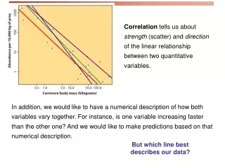
Correlation tells us about strength (scatter) and direction of the linear relationship between two quantitative variables. In addition, we would like to have a numerical description of how both variables vary together. For instance, is one variable increasing faster than the other one? And we would like to make predictions based on that numerical description. But which line best describes our data?
Response (dependent) variable: blood alcohol content y x Explanatory (independent) variable: number of beers Recall: explanatory and response variables A response variablemeasures or records an outcome of a study - the endpoint of interest in the study. An explanatory variableexplains changes in the response variable. Typically, the explanatory or independent variable is plotted on the x axis, and the response or dependent variable is plotted on the y axis.
Some plots don’t have clear explanatory and response variables. Do calories explain sodium amounts? Does percent return on Treasury bills explain percent return on common stocks?
The regression line • A regression line is a straight line that describes how a response variable y changes as an explanatory variable x changes - the description is made through the slope and intercept of the line. • We often use a regression line to predict the value of y for a given value of x; the line is also called the prediction line, or the least-squares line, or the best fit line. • In regression, the distinction between explanatory and response variables is important - if you interchange the roles of x and y, the regression line is different. y-hat is the predicted value of y b1 is the slope b0 is the y-intercept
Distances between the points and line are squared so all are positive values. This is done so that distances can be properly added… The regression line The least-squares regression line is the unique line such that the sum of the squares of the vertical (y) distances between the data points and the line is as small as possible ("least squares")
How to: First we calculate the slope of the line, b1; from statistics we already know: r is the correlation. sy is the standard deviation of the response variable y. sx is the the standard deviation of the explanatory variable x. Once we know b1, the slope, we can calculate b0, the y-intercept: Where and are the sample means of the x and y variables Typically, we use the TI-83 or JMP (Analyze -> Fit Y by X -> under the red triangle, Fit Line) to compute the b's, rarely using the above formulas…
JMP output the regression line intercept estimate is b0 slope estimate b1 is the coefficient (Estimate) of the NEA term
The equation completely describes the regression line. To plot the regression line you only need to plug two x values into the equation, get the two y's, and draw the line that goes through those points. Hint: The regression line always passes through the mean of x and the mean of y. BAC= -.013 + .018 * No. Beers Usually we let JMP draw the regression line as here…
Hubble telescope data about galaxies moving away from earth: These two lines are the two regression lines calculated either correctly (x = distance, y = velocity, solid line) or incorrectly (x = velocity, y = distance, dotted line). Unlike in Correlation, the distinction between explanatory and response variables is crucial in Regression. If you exchange y for x in calculating the regression line, you will get a different line. Regression examines the distance of all points from the linein the y direction only.
Making predictions The equation of the least-squares regression allows you to predict y for any xwithin the range studied - be careful about extrapolation! Confirm the regression line's equation below using JMP Nobody in the study drank 6.5 beers, but by finding the value of from the regression line for x = 6.5 we would expect a blood alcohol content of 0.104 mg/ml.
= - ˆ y 0 . 125 x 41 . 4 = - ˆ y 0 . 125 x 41 . 4 (in 1000s) There is a positive linear relationship between the number of powerboats registered and the number of manatee deaths. The least squares regression line has the equation: Thus if we were to limit the number of powerboat registrations to 500,000, what could we expect for the number of manatee deaths? Roughly 21 manatees.
!!! !!! Extrapolation Extrapolation is the use of a regression line for predictions outside the range of x values used to obtain the line. This can be a very stupid thing to do, as seen here. Height in Inches Height in Inches
The y intercept Sometimes the y-intercept is not realistically possible. Here we have negative blood alcohol content, which makes no sense… But the negative value is correct for the equation of the regression line. There is a lot of scatter in the data, and the slope and intercept of the line are both estimates. We'll see later the y-intercept is probably not "significantly different from zero" y-intercept shows negative blood alcohol
r = 0.87 r 2 = 0.76 Coefficient of determination, r 2 r 2 representsthe percentage of the variation in y(vertical scatter from the regression line) that can be explained by the regression of y on x.r 2 is the ratio of the variance of the predicted values of y (y-hats - as if no scatter around the line) to the variance of the actual values of y. r 2, the coefficient of determination, is the square of the correlation coefficient.
r = 0.87 r 2 = 0.76 y is entirely independent of what value x takes on: r 2 = 0 r = 0 r 2 = 0 Here the regression of y on x explains only 76% of the variation in y. The rest of the variation in y (the vertical scatter, shown as red arrows) must be explained by something other than the line. r = -1 r 2 = 1 Changes in x explain 100% of the variation in y. Y can be entirely predicted for any given value of x.
Here are two plots of height (response) against age (explanatory) of some children. Notice how r2 relates to the variation in heights... r=0.994, r-square=0.988 r=0.921, r-square=0.848
Body weight and brain weight in 96 mammal species r = 0.86, but this is misleading. The elephant is an influential point. Most mammals are very small in comparison. Without this point, r = 0.50 only. Now we plot the log of brain weight against the log of body weight. The pattern is linear, with r = 0.96. The vertical scatter is homogenous → good for predictions of brain weight from body weight (in the log scale).
Homework: • You should have read through section 2.3, carefully reviewing what you know about lines from your algebra course…Go over Examples 2.18-2.21 in some detail so you understand them! • Do #2.66, 2.71-2.73, 2.78, 2.82, 2.83 Use JMP to make the scatterplots, describe the association you see between the two variables, and then let JMP calculate the intercept and slope and r-square for the regression line. Explain what the slope and intercept mean in the context of the specific problem. Also, practice doing the above computations with the TI-83 - I'll help you get started with the calculator in class…