Temperature
Learn about temperature, different temperature scales (Fahrenheit, Celsius, Kelvin), conversions between scales, and how temperature is measured using thermometers.

Temperature
E N D
Presentation Transcript
Temperature The property of an object that determines the direction of heatenergy (Q) transfer to or from other objects.
Temperature Scales • Three Common Scales are used to measure temperature: 1. Fahrenheit Scale (°F) 2. Celsius (Centigrade) Scale(°C) 3. Kelvin Scale (K)
Fahrenheit Scale (°F) • Used widely in the U.S. Divides the difference between freezing & boiling point of water at sea level into 180 steps. Celsius (Centigrade) Scale(°C) • Used almost everywhere else in the world. Divides the freezing to boiling continuum into 100 equal steps.
Kelvin Scale (K) • Used by scientists. Created by Lord Kelvin. Starts with T = 0 K “Absolute Zero”.
Some Physics History! (Interesting to me!) • There have also been many other temperature scales used in the past! Among these are: 1. Rankine Scale (°Ra). 2. Réaumur Scale(°Ré) 3. Newton Scale (°N). 4. Delisle Scale (°D). 5. Rømer Scale. (°Rø). Some Conversions:
Temperature Scale Comparisons • Boiling Point of Water 212°F = 100°C = 373.15 K • Melting Point of Ice 32°F = 0°C = 273.15 K • “Absolute Zero” -459.67°F = -273.15°C = 0K • Average Human Body Temperature: 98.6°F = 37°C = 310.16 K • Average Room Temperature: 68°F = 20°C = 293.16 K
Common Conversions Celsius to Fahrenheit: F° = (9/5)C° + 32° Fahrenheit to Celsius: C° = (5/9)(F° - 32°)
The Kelvin ScaleSometimes Called the Thermodynamic Scale • The Kelvin Scale was created by Lord Kelvin to eliminate the need for negative numbers in temperature calculations. The Kelvin Scale isdefinedas follows: 1.The degree size isidenticalto that on the Celsius scale. 2.The temperature in Kelvin degrees at the triple point of water is DEFINED to be Exactly 273.16 K
How is Temperature Measured? • Of course,temperature is measured using a • Thermometer!
How is Temperature Measured? • Of course,temperature is measured using a • Thermometer! • Thermometer Any object that has a property characterized by a • Thermometric Parameter
How is Temperature Measured? • Of course,temperature is measured using a • Thermometer! • Thermometer Any object that has a property characterized by a • Thermometric Parameter • Thermometric ParameterAny parameter X, that varies in a known (calibrated!) way with temperature. Measure the value of X at TWO fixed points of temperature & interpolate & extrapolate as needed.
X • X2 X1 • Xm FP2 FP1 T Error! • Thermometric ParameterAny parameter X, that varies in a known (calibrated!) way with temperature. Measure the value of X at TWO fixed points of temperature & interpolate & extrapolate as needed. Two (or more) reference points can result inerrorswhen extrapolating outside of their range!!
Ranges of Various Types of Thermometers V P or V n.b.p. “normal boiling point”
Reference Points for Temperature Scales Some Brief History. • Daniel Fahrenheit (1724) • Ice, water & ammonium chloride mixture = 0 °F • Human body = 96 °F (now taken as 98.6 °F) • Anders Celsius (1742) • Originally: Boiling point of water = 0 ºC! • Melting point of ice = 100 ºC! • The Scale was later reversed! • This scale was originally • called “centigrade”
Pt & RuO2 Resistance Thermometers t T For 0 ºC < T < 850 ºC Blundell & Blundell, Concepts in Thermal Physics(2006)
Spectral Distribution of Thermal Radiation (Planck Distribution Law) Radiation Energy Density Infrared UV-Visible
Fixed Temperature Reference Points Melting points of metals and alloys Reports on Progress in Physics, vol. 68 (2005) pp. 1043–1094
Temperature Scale (with Single Fixed Point) • Defining a temperature scale with a single fixed point • requires a linear (monotonic) relationship between a • Thermometric Parameter X & the • Temperature Tx: X = cTx, (c is a constant) • By international agreement in 1954, • The KelvinorThermodynamic • Temperature Scale • uses the triple point (TP) of water as the fixed point. There, • The temperature is defined • (notmeasured!) to be Exactly273.16 K
• The Triple Point of Water At the triple point of water: gas, solid & liquid all co-exist at a pressure of 0.0006 atm.
Temperature Scale with a Single • Fixed Point • For Thermometric Parameter X at • any temperature Tx: So, • What variable should be measured to use the • thermodynamic temperature scale?
Gas P, V Unknown T TP = 273.16K The Ideal Gas Temperature Scale The Ideal Gas Law: Hold V & n constant!
Defining the Kelvin & Celsius Scales • “One Kelvin degree is (1/273.16) of the • temperature of the triple point of water.” • Named after William Thompson (Lord Kelvin). • Relationship between °C and K • °C = K - 273.15 • Note that careful measurements find that at • 1 atm. water boils at 99.97 K above the • melting point of ice (i.e. at 373.12 K) so • 1 K is not exactly equal to 1° Celsius!
The 2nd Law Tells Us That: Heat flows from objects at high temperature to objects at low temperature because this process increases disorder & thus it increases the entropy of the system.
Heat Reservoirs • The following discussion is similar to that for which the Energy Distribution Between Systems in Equilibriumwas discussed & the conditions for equilibrium were derived. A1 A2 • Recall: We considered 2 macroscopic systems A1,A2,interacting & in equilibrium. The combined system • A0 = A1 +A2, was isolated. E2 = E - E1 E1 • Then, we found the most probable energy of systemA1, using the fact that the probability finding of A1 with a particular energy E1is proportional to the product of the number of accessible states of A1times the number of accessible states of A2, Consistent with Energy • Conservation: E = E1 + E2
The probability finding of A1 with a particular energy E1is proportional to the number of accessible states of A1times the number of accessible states of A2, • Consistent with Energy Conservation: E = E1 + E2. • That is, it is proportional to • Using differential calculus to find the E1 that maximizes Ω(E1, E – E1) resulted in statistical definitions of both the Entropy S & the Temperature Parameter: • It also resulted in the fact that the equilibrium condition for A1 & A2is • that the two temperatures are equal!
Consider a special caseof the situation just reviewed. A1 & A2are interacting & in equilibrium. But, • A2is a Heat Reservoir or Heat Bath for A1. • Conditions for A2to be a Heat Reservoir for A1: • E1 <<< E2, f1 <<< f2 • Terminology in some books:A2 is “large” compared to A1 • Assume that A2absorbs a small amount of heat energy Q2from A1. • Q2 = E2 E1 • The change in A2’s entropy in this process is • S2 = kB[lnΩ(E2 + Q2) – lnΩ(E2)] • Expand S2 in a Taylor’s Series for • small Q2& keep only the lowest order • term. Also use the temperature • parameter definition.
S2 = kB[lnΩ(E2 + Q2) – lnΩ(E2)] • Expand S2 in a Taylor’s Series for small Q2& keep only the lowest order term. Use the temperature parameter definition & connection with absolute temperature T: • l • This results in S2 kBQ2. Also note that since the two systems are in equilibrium, T2 = T1 T so: • S2 [Q2/T] • In another notation this is: • S' [Q'/T]
Summary: Heat Reservoirs • For a system interacting with a heat reservoir at temperature T & giving heat Q'to the reservoir, the change in the entropy of the reservoir is: • S' [Q'/T] • For an infinitesimal amount of heat đQ exchanged, the differential change in the entropy is: • dS = [đQ/T]
The 2nd Law of Thermodynamics: • Heat flows from high temperature objects to low • temperature objects because this increases the disorder • & thus the entropy of the system. We’ve shown that, • For a system interacting with a heat reservoir at temperatureT & exchanging heatQ with it, the entropy change is:
External Parameter Dependence of Ω • The following is similar to our previous discussion, where the Energy Distribution Between Systems in Equilibriumwas discussed & the conditions for equilibrium were derived. • Recall:We considered 2 macroscopic systems • A1,A2,interacting & in equilibrium. The combined system A0 = A1 +A2, was isolated. A2 A1 • Now:Consider the case in which A1 & A2are also characterized by external parameters x1 & x2. x2 x1 E2 = E - E1 E1 • As discussed earlier, corresponding to x1 & x2, there are generalized forces X1 & X2.
In earlier discussion, we found the most probable energy of systemA1, using the fact that the probability finding of A1 with energy E1is proportional to the product of the number of accessible states of A1times the number of accessible states of A2, Consistent with Energy Conservation: E = E1 + E2 • That is, it is proportional to • Using calculus to find E1 that maximizes Ω(E1, E – E1) resulted in statistical definitions of the Entropy S & the Temperature • Parameter. • Another result is that the equilibrium condition for A1 & A2is that the temperatures are equal!
When external parameters are present, the number of accessible states Ω depends on them & on energyE. • Ω = Ω(E,x) • In analogy with the energy dependence discussion, the probability finding of A1 with a particular external parameter x1is proportional to the number of accessible states of A1times the number of accessible states of A2. • That is, it is proportional to • Ω(E1,x1;E2,x2) = Ω(E1,x1)Ω(E - E1,x2)
The probability finding of A1 with a particular external parameter x1is proportional to the number of accessible states of A1times the number of accessible states of A2. • Ω(E1,x1;E2,x2) = Ω(E1,x1)Ω(E - E1,x2) • Using differential calculus to find the x1 that maximizes Ω(E1,x1;E2,x2) results in a statistical definition of • The Mean Generalized Force <X> • <X> ∂ln[Ω(E,x)]/∂x (1) • or <X> = (kBT)∂ln[Ω(E,x)]/∂x (2) • In terms of Entropy S: • <X> = T[∂S(E,x)]/∂x (3) • (1) ((2) or (3)) is called an Equation of Statefor system A1. Note that there is an Equation of State for each different external parameter x.
Summary • For interacting systems with an external parameter x, at equilibrium • The Mean Generalized Force <X> is • <X> ∂ln[Ω(E,x)]/∂x (1) • Or <X> = (kBT)∂ln[Ω(E,x)]/∂x (2) • <X> = T ∂S(E,x)]/∂x (3) • (1) ((2) or (3)) is an Equation of Statefor system A1. There is an Equation of State for each different external parameter x.