Images and M ATLAB
570 likes | 765 Views
Images and M ATLAB. Digital Image Processing. Image Basics w.r.t. Matlab Image Display. Matlab and Images. MATLAB is a data analysis software package with powerful support for matrices and matrix operations Command window Reads pixel values from image Creates a figure on the screen

Images and M ATLAB
E N D
Presentation Transcript
Images and MATLAB Digital Image Processing
Matlab and Images • MATLAB is a data analysis software package with powerful support for matrices and matrix operations • Command window • Reads pixel values from image • Creates a figure on the screen • Display matrix as an image • Turns on pixel values in the figure • Pixel values appear at the bottom of the figure {Pixel info: (c,r) [r,g,b]} • We may measure pixel distance by replacing impixelinfo with imdistline
>> figure, imshow(‘trees.tif’) >> em = imread(‘trees.tif’); >> figure, imshow(em) Indexed Color Images (1/2) Ch2-p.25
>> [em, emap] = imread(‘trees.tif’); >> figure, imshow(em, emap) Indexed Color Images (2/2) • Information about Your Image • A great deal of information can be obtained with theimfinfofunction Ch2-p.26
Data Types and Conversions (1/2) Ch2-p.28
Data Types and Conversions (2/2) Ch2-p.28
Images Files and Formats • You can use MATLAB for image processing very happily without ever really knowing the difference between GIF, TIFF, PNG, etc. • However, some knowledge of the different graphics formats can be extremely useful in order to make a reasoned decision Ch2-p.29
Images Files and Formats (1/3) • Header information • This will, at the very least, include the size • of the image in pixels (height and width) • It may also include the color map, compression used, and a description of the image Ch2-p.29
Images Files and Formats (2/3) • The imread and imwrite functions of MATLAB currently support the following formats • JPEG These images are created using the Joint PhotographicsExperts Group compression method • TIFF A very general format that supports different compression methods, multiple images per file, and binary, grayscale, truecolor, and indexed images Ch2-p.30
Images Files and Formats (3/3) • GIF • A venerable format designed for data transfer. It is still popular and well supported, but is somewhat restricted in the image types it can handle • BMP • Microsoft Bitmap format has become very popular and is used by Microsoft operating systems • PNG, HDF, PCX, XWD, ICO, CUR Ch2-p.30
A Hexadeciaml Dump Function Ch2-p.30
Vector versus Raster Images • We may store image information in two different ways • Vector images: a collection of lines or vectors • Raster images: a collection of dots • The great bulk of image file formats store images as raster information Ch2-p.31-32
A Simple Raster Format • As well as containing all pixel information, an image file must contain some header information • this must include the size of the image, but may also include some documentation, a color map, and the compression used • e.g. PGM format was designed to be a generic format used for conversion between other formats Ch2-p.32
Microsoft BMP Header (1/3) Ch2-p.33
Microsoft BMP Header (2/3) Ch2-p.33
Microsoft BMP Header (3/3) • The image width is given by bytes 18–21; they are in the second row 42 00 00 00 • (due to little endian) To find the actual width, we reorder these bytes back-to-front: 00 00 00 42 • The size of the image is then computed: • Width: (4×161)+(2×160) = 66 • Height: (1×161)+(F×160) = 31 (1F 00 00 00 => 00 00 00 1F) Ch2-p.34
Image File Format: GIF • Colors are stored using a color map. The GIF specification allows a maximum of 256 colors per image • GIF doesn’t allow binary or grayscale images, except as can be produced with RGB values • The pixel data is compressed using LZW (Lempel-Ziv-Welch) compression • The GIF format allows multiple images per file. This aspect can be used to create animated GIFs Ch2-p.34-35
Image File Format: PNG • The PNG format has been more recently designed to replace GIF and to overcome some of GIF’s disadvantages • Does not rely on any patented algorithms, and it supports more image types than GIF • Supports grayscale, true color, and indexed images • Moreover, its compression utility, zlib, always results in genuine compression Ch2-p.35
Image File Format: JPEG • The JPEG algorithm uses lossy compression, in which not all the original data can be recovered Ch2-p.35-36
Image File Format: TIFF (1/2) • Comprehensive image formats, excellent for data exchange • Can store multiple images per file • Allows different compression routines and different byte orderings • Allows binary, grayscale, truecolor or indexed images, and opacity or transparency Ch2-p.36-37
Image File Format: TIFF (2/2) • This particular image uses the little-endian byte ordering • The first image in this file (which is in fact the only image), begins at byte • Because this is a little-endian file, we reverse the order of the bytes: 00 01 01 E0. This works out to 66016 Ch2-p.37
Image File Format: DICOM • DICOM (Digital Imaging and Communications in Medicine) • Like GIF, may hold multiple image files • May be considered as slices or frames of a three dimensional object • The DICOM specification is huge and complex. Drafts have been published on the World Wide Web Ch2-p.37-38
Files in MATLAB • Which writes the image stored in matrix X with color map map (if appropriate) to file filename with format fmt • Without the map argument, the image data is supposed to be grayscale or RGB e.g. Ch2-p.38
Introduction • We take a closer look at the use of the imshow function • We look at image quality and how that may be affected by various image attributes • For human vision in general, the preference is for images to be sharp and detailed Ch3-p.41
Basics of Image Display (1/6) • There are many factors that will affect the display • ambient lighting • the monitor type and settings • the graphics card • monitor resolution
Basics of Image Display (2/6) • This function image simply displays a matrix as an image Incorrect due to irrelevant colormap employed by the image() function. Ch3-p.42
Basics of Image Display (3/6) • To display the image properly, we need to add several extra commands to the image line
Basics of Image Display (4/6) • We may to adjust the color map to use fewer or more colors; however, this can have a dramatic effect on the result Ch3-p.43
Basics of Image Display (5/6) • use imread to pick up the color map • map is <256×3 double> in the workspace Ch3-p.43
Basics of Image Display (6/6) • True color image will be read (by imread) as a three-dimensional array • In such a case, image will ignore the current color map and assign colors to the display based on the values in the array Ch3-p.43
The imshowFunction (1/5) • We have two choices with a matrix of type double: • Convert to type uint8 and then display • Display the matrix directly • imshow will display a matrix of type double as a grayscale image (matrix elements are between 0 and 1) Ch3-p.44
The imshow Function (3/5) • We can convert the original image to double more properly using the function im2double • If we take cd of type double, properly scaled so that all elements are between 0 and 1, we can convert it back to an image of type uint8 in two ways:
The imshow Function (4/5) • BINARY IMAGES MATLAB have a logical flag, where uint8 values 0 and 1 can be interpreted as logical data • Check c1 with whos
>> imshow(cl) >> imshow(uint8(cl)) The imshow Function (5/5) Ch3-p.47
Bit Planes (1/3) • Grayscale images can be transformed into a sequence of binary images by breaking them up into their bitplanes • The zeroth bit plane • the least significant bit plane • The seventh bit plane • the most significant bit plane
Bit Planes (2/3) • We start by making it a matrix of type double; this means we can perform arithmetic on the values
Spatial Resolution (1/3) • The greater the spatial resolution, the more pixels are used to display the image • We can experiment with spatial resolution with MATLAB’s imresizefunction
Spatial Resolution (2/3) imresize(imresize(x, factor, ‘nearest’), factor, ‘nearest’);
Quantization (1/3) • Uniform quantization
Quantization (2/3) • To perform such a mapping in MATLAB, we can perform the following operations, supposing x to be a matrix of type uint8 • There is, a more elegant method of reducing the grayscales in an image, and it involves using the grayslice function
Dithering (1/5) • DITHERING In general terms, refers to the process of reducing the number of colors in an image • Representing an image with only two tones is also known as halftoning • Dithering matrix • D or D2 is repeated until it is as big as the image matrix, when the two are compared
Dithering (2/5) • Suppose d(i, j)is the matrix obtain by replicating the dithering matrix, then an output pixel p(i, j)is defined by